Note
Need help? Please let us know in the UMEP Community.
4.6. Urban Energy Balance: GQF
- Contributor
Name
Institution
Andy Gabey
Reading
Izzy Capel Timms
Reading
Sue Grimmond
Reading
- How to Cite
Gabey A, S Grimmond, I Capel-Timms 2018: Anthropogenic Heat Flux: advisable spatial resolutions when input data are scarce Theoretical and Applied Climatology https://doi.org/10.1007/s00704-018-2367-y
Lindberg F, CSB Grimmond, A Gabey, B Huang, CW Kent, T Sun, NE Theeuwes, L Järvi, H Ward, I Capel-Timms, YY Chang, P Jonsson, N Krave, DW Liu, D Meyer, KFG Olofson, JG Tan, D Wästberg, L Xue, Z Zhang 2018: Urban multiscale environmental predictor (UMEP) - An integrated tool for city-based climate services Environmental Modelling and Software 99, 70–87 10.1016/j.envsoft.2017.09.020
- Introduction
- Dialog box
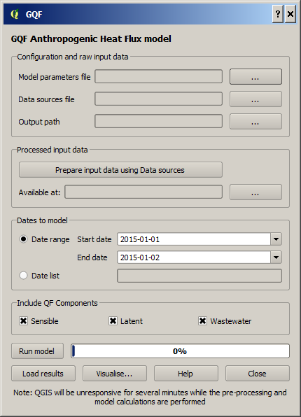
Fig. 4.13 Diolag for the GQF model
- Dialog sections
- The model run is configured using the dialog box:
Start date and end date: The first and final dates for which the model should be run.
Output areas: Two options are currently available: Local authority areas and 1km grid. These select the spatial units of the model calculations.
Include QF components: The components of anthropogenic heat flux for the model to include in calculations.
Output path: A directory that houses model outputs.
- Model outputs
- Example map
The total anthropogenic heat flux for the first time step is displayed in QGIS to demonstrate model output and the output areas. In order for these areas to be displayed correctly, the coordinate reference system must be selected. The QGIS “Select CRS” screen will appear, and EPSG 27700 (British National Grid) must be chosen.
The layer displaying model output also contains the other contributions to QF (e.g. car transport). These can be visualised using standard QGIS methods of styling the layer according to the selected component, or inspecting the layer attributes table.
- CSV files
A CSV file is generated for each of the 19 contributions to QF (e.g. car travel, wastewater heating) and the total QF. Each file contains a column per output area (shown in the example map) and a row per time step. These are labelled accordingly. The filenames are abbreviated where necessary for compatibility, with the following convention used:
El
Electricity
Gas
Gas
Dm
Domestic use
Id
Industrial use
Tspt
Transport
Unre
Unrestricted electricity (non-Economy 7)
Eco7
Economy 7 electricity
Everything
Grand total QF across all sources
A “pickled” Python data object containing the results is also saved in the local temporary folder for future use with other UMEP components.
- References
Iamarino M, Beevers S & Grimmond CSB (2012) High-resolution (space, time) anthropogenic heat emissions: London 1970-2025 International J. of Climatology 32, 11, 1754-1767
Gabey A, S Grimmond, I Capel-Timms 2018: Anthropogenic Heat Flux: advisable spatial resolutions when input data are scarce Theoretical and Applied Climatology https://doi.org/10.1007/s00704-018-2367-y
Lindberg F, CSB Grimmond, A Gabey, B Huang, CW Kent, T Sun, NE Theeuwes, L Järvi, H Ward, I Capel-Timms, YY Chang, P Jonsson, N Krave, DW Liu, D Meyer, KFG Olofson, JG Tan, D Wästberg, L Xue, Z Zhang 2018: Urban multiscale environmental predictor (UMEP) - An integrated tool for city-based climate services Environmental Modelling and Software 99, 70–87 10.1016/j.envsoft.2017.09.020