LQF provides a method to calculate the anthropogenic heat flux. It uses
wide-area energy consumption and vehicle ownership values, and uses and
higher-resolution residential population data estimate the heat flux
from buildings, transport and human metabolism at 60 minute intervals at
the spatial resolution of the population data.
Energy and vehicle use are assumed to be correlated to residential
(night-time) populations
Temporal resolution is maximised by applying empirically measured
diurnal, day-of-week and seasonal variations to the data.
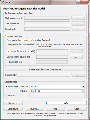
The main user interface allows the user to select the temporal extent of
the model run, and the configuration files. The configuration files
describe model assumptions and the library of available data files.
1: Specify model configuration files and output path:
LQF needs spatial and temporal information about the population, energy consumption and transport in order to model QF at high temporal and spatial resolution:
Model parameters file: Fortran-90 namelist file containing numerical parameters required in model calculations
Data sources file: Fortran-90 namelist file that contains the locations of spatial and temporal input files used by the model
Output Path: Directory into which Model outputs and associated data will be stored. Any existing files will be overwritten.
2: Input data is pre-processed:
Before it can be used in the model, the wide-area energy use, vehicle ownership and population data in the data sources file must be (dis)aggregated using local population data to match the chosen output areas.
Data is processed using the Prepare input data using data sources button. This performs disaggregation and saves the output files to the /DownscaledData/ subfolder of the chosen model output directory. This step can take up to several hours, during which QGIS will not respond to input.
If processed input data already exists elsewhere it can be used instead by specifying the path using the Available at: box. The processed files are copied to the /DownscaledData/ subfolder of the chosen model output directory.
Optional: Extra disaggregation uses an additional set of inputs so the data can be disaggregated to a higher spatial resolution:
Land cover fractions: Land cover fractions calculated using the UMEP land cover classifier in the pre-processing toolbox.
Corresponding polygon grid: The ESRI shapefile grid of polygons represented by the land cover fractions.
Grid cell ID field: The field of the polygon grid shapefile that contains a unique identifier for each cell. This is used to cross-reference model outputs.
3: Choose temporal domain:
Dates to model (outputs are produced at 60-minute intervals). Either:
Date range: The first and final dates are specified and the whole period is simulated.
Date list: A comma-separated list of dates in YYYY-mm-dd format (e.g. 2015-01-02, 2016-03-05, 2014-05-03) is provided. These dates are simulated in their entirety.
4: Run model and visualise results:
The Run Model button executes the model, which applies the temporal disaggregations and calculates QF components in each output area. This takes up to several hours for high resolution or long study periods. During this time QGIS will not respond to input.
Results are visualised using the Visualise… button
Previous model results are retrieved using the Load Results button, which allows a previous model output folder to be selected.
Data are ready for use in QF calculations after this point
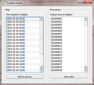
A simple visualisation tool accompanies the model which produces maps and time series plots of the available data.
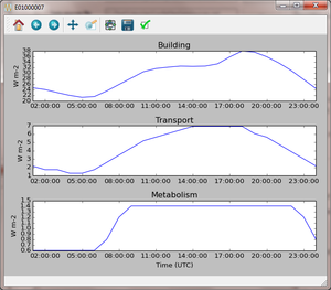
Time series plots
One plot per output area is produced for all of the time steps present in the model output directory, showing the three QF components on separate axes. To plot a time series, select the output area of interest and click the “Show plot” button. The plot areas can be manipulated and graphs exported using the tools in the plot window.
Maps
One map per QF component and time step is produced, coloured on a logarithmic scale according to the QF value in each output area. One or more LQF time steps is selected in the list, and every QF component is displayed for each date in the QGIS window by pressing “Add to canvas”.
Note: Rendering maps may take several minutes for high-resolution model results.
Model outputs are stored in the /ModelOutput/ subdirectory of the
selected model output directory. A separate data file is produced for
each time step of the model run. Each file contains four columns (one
each for total, building, transport and metabolism) and a row for each
output area.
Output files are timestamped with the pattern
LQFYYYYmmdd_HH-MM.csv, with times stated in UTC.
YYYY: 4-digit year
mm: 2-digit month
dd: 2-digit day of month
HH: 2-digit hour (00 to 23)
MM: 2-digit minute
The first model output is labelled 01:00UTC and covers the period
00:00-01:00 UTC.
Each data file is in comma-separated value (CSV) format
If pre-processing of the input data has taken place, the Disaggregated
energy, transport and population shapefiles are stored in the
/DownscaledData/ subdirectory of the model outputs, with filenames
that reflect the time period they represent. This folder can be used as
the source of processed input data in future runs to save time, provided
that the data sources file has not changed.
If previously processed input data are being used, these are copied to
the /DownscaledData/ subdirectory of the current model run
Several log files are saved in the /Logs/ subdirectory. The logs are
intended to help interpretation of model outputs by providing a
traceable history of why a particular spatial or temporal disaggregation
value was looked up.
The steps taken to disaggregate spatial data, including which
attributes were involved
The day of week and the time of day that was returned from each
diurnal and annual profile data source when it was queried with a
particular model time step.
Input data consists of spatial and temporal information, a lookup table
for vehicle fuel efficiency and (optionally) land use cover data to
further enhance the spatial resolution of the model output.
An internal database contains nation-level parameters. These are
disaggregated and downscaled based on residential population data. Any
output areas spatially outside a territory will be labelled as belonging
to no nation, and therefore receive zero vehicles, energy consumption or
metabolism.
The database contains the following data for each country. Some of these
are time varying, which values stored for each year that data is
available (1950 onwards). The data can be added to using standard SQL
tools such as SQLite browser, the pandas package in Python or
open-source programming tools. Data can be added for any or all
time-varying quantities, and non-consecutive years are permitted. The
entries are as follows:
Attribute
Description
Units
kwh_year
Total annual primary energy consumption (time-varying)
kWh per year
motorcycles
Total motorcycle ownership (time varying)
Per 1,000 people
cars
Total passenger car ownership (time varying)
Per 1,000 people
freight
Total freight vehicles (time varying)
Per 1,000 people
ecostatus
World Bank national income classification (1 to 4, 1 being highest)
summer_cooling
Whether summer cooling is a significant impact on energy consumption (1=Yes, 0=No)
wake_hour
Time when 50% of the population has woken up in the morning
Hour of day (local time)
sleep_hour
Time when 50% of the population has gone to sleep at night
Hour of day (local time)
transition_time
Timescale over which waking and sleeping occurs
Hours
population
Total population (time-varying)
fixedHolidays
Days of the year that contain fixed public holidays for each country (e.g. December 25 in the UK)
DOY (non-leap year. Adjusted values used when leap year modelled)
weekendDays
The days of the week that are assumed as weekends in each country
1 (weekend) or 0 (weekday)
weekendCycles
Country-specific diurnal variation for weekend building energy consumption and traffic flow
Local time
weekdayCycles
Country-specific diurnal variation for weekday building energy consumption and traffic flow
An ESRI shapefile containing spatially resolved population data. This is
used to disaggregate the wide-area totals and estimate metabolism across
the study area.
Since population data are key to the model method, it is important to
use the finest available spatial scale.
The model must output results for a consistent set of spatial units,
so the populations are assigned to the model output areas based on
how much each spatial unit of population is intersected each output
area. It is recommended that a population shapefile is chosen as
the output areas.
The field containing the population must be labelled “Pop” in the
shapefile attributes
Temporal data allows the annualised data provided by the shapefiles to
be temporally disaggreated into time series. LQF requires daily and
hourly information:
Daily information: The mean daily temperature (degrees Celsius)
for the region being studied, covering the period of study. The model
estimates day-to-day changes in building energy consumption based on
the daily mean temperature. The temperature input file for each year
is provided by a file with 365 (or 366) entries.
Hourly information: Template diurnal cycles at 60-minute
intervals for total energy consumption, total traffic flow, metabolic
heat emitted per person and the proportion of the population emitting
this heat.
Variations of these cycles for different days of week
Variations of the above at different times of year (if
available)
Metabolism is based purely on data in the LQF database and can’t be
overridden. The LQF database contains one default diurnal profile for
traffic flow and building energy consumption, but these should be
overridden with local data files whenever possible:
QF component
File description(s)
Size of file
Transport
Traffic flows for each vehicle type during each day of the week
7 days * 24 hours * N seasons
Building
Building energy consumption during each day of the week
7 days * 24 hours * N seasons
Each temporal file contains headers that store metadata used by the
model to interpret the data:
The time zone represented by the file
(“UTC”
or of the style “Europe/London”). If “UTC” is specified, then values
must be explicitly provided for each daylight savings regime to
capture shifts in human behaviour. Note that the model outputs are
always UTC, with the necessary conversion taking place in the
software.
The start and end dates of the period represented by the data. This
allows seasonality to be captured.
Ideally these files contain data taken from the period being modelled,
but this is not always practical. In this case, temporal profile data
from the most recent available year is looked up for the same day of
week (taking into account public holidays), season and daylight savings
regime if applicable. Different variants are used for traffic, energy
and metabolism, and each of these is described below.
This file records daily air temperature, from which the model estimates
the response in building energy consumption. These are expressed in
degrees Celsius.
The file consists of two columns. The first is the day of year; the
second is the temperature. The file must contain values for the days
from StartDate to EndDate (inclusive), and the column and row headers
must be identical to those shown.
The same file format is used for both traffic flow and building energy
consumption. Each file contains 7 days of data at 1 hour resolution (168
rows). The first row represents the period 00:00-01:00 on Monday
morning, and the final row represents 23:00-00:00 on Sunday Evening
(into Monday).
The following header lines must be present:
Season: A name for the period represented by each column.
Start Date: The first day of the period (e.g. season) represented
by the data
End Date: The final day of this period
Notes:
Periods are not allowed to overlap
The units of measurement are not important: The values within a given
day are normalised after they are loaded into the model software
The example below shows the first 24 rows of a file that contains
entries for the 4 quarters of 2014. Any number of seasons/periods of
year can be added to a single file, and multiple files can be added.
Metabolic activity is calculated based on the parameters in the
database, which do not change over time (unlike energy consumption,
population and vehicle ownership).
The populace is assumed to emit more metabolic energy during waking
hours than during sleep, with a linear transition between these two
states based on the time people generally wake and sleep in each
country. A study area spanning national boundaries therefore shows
spatial variation in metabolic activity in the morning and evening if
the countries have different waking and sleeping hours in the LQF
database.
The model calculates fluxes for any date provided there is temporal data
for the corresponding time of year. If daily temperatures and/or diurnal
cycles are not available for the date being modelled, a series of
lookups is performed on the available temporal data to find a suitable
match. This process accounts for changes in public holidays, leap years
and changing DST switch dates.
For diurnal cycle data, the lookup operates by building and then
reducing a shortlist of cycles that may be suitable:
Based on the modelled time step, cycles from a suitable year are
added to the shortlist. A year is deemed suitable if it contains data
covering the time of year being modelled
If the modelled year is later than available data, the latest
suitable year is used
If the modelled year is earlier than the available data, the
earliest suitable year is used
The modelled day of week is established (set to Sunday if a public
holiday)
The lookup date is set as the same day of week, month and time of
month as the modelled date, but in the year identified as suitable.
This operation sometimes causes late December dates to become
early January. Such dates are moved into the final week of
December.
The daylight savings time (DST) state is identified for the lookup
date, based on the time shift at noon.
Down-select the available cycles based on the DST state
(user-provided diurnal profile files only, when timezone of the
modelled city is not the same as that in the profile file):
If the cycles are not provided in the local time of the city being
modelled, the search is narrowed to those cycles for
periods/seasons matching this DST state
If the cycles are provided in the local time of the city being
modelled, all periods/seasons are available
Remove any cycles that do not contain the necessary day of week from
the shortlist
The most recent cycle with respect to the lookup date is used
The same process is used to identify a relevant daily temperature,
except in this case a single value is looked up instead of a cycle and
each day of the year is its own season to improve resolution.
This is optional. It assigns transport, building and metabolism heat
fluxes to only those regions of that map with compatible land covers.
Since land cover fraction data are often available at high spatial
resolution, this increases the resolution of the model outputs beyond
the output areas that were specified initially.
Each model output area is divided into a number of “refined output
areas” (ROAs). The land cover fraction lists the proportion of each ROA
occupied by:
Water
Paved surfaces
Buildings
Soil
Deciduous Trees
Coniferous Trees
Grass
The GQF user interface requires two input files for this process.
Corresponding polygon grid: The ESRI shapefile grid of polygons
represented by the land cover fractions. This is a required input for
the UMEP land cover classifier.
‘’Note that this feature may be very slow and memory limitations may
cause it to fail or produce very large output files.’’
The overall building, transport and metabolic QF components in
an MOA are attributed to each ROA based on a set of weightings that
associate land cover classes with QF components.
A fixed set of weightings determines the behaviour of this routine and
ensure the following principles are satisfied:
Transport heat flux only occurs on paved areas (roads)
Building heat flux only occurs where there are buildings
Metabolic energy reflects the distribution of people between indoor
and outdoor environments
Land cover class
Weightings (columns must sum to 1)
QF,B
QF,M
QF,T
Building
1
0.8
0
Paved
0
0.05
1
Water
0
0.0
0
Soil
0
0.05
0
Grass
0
0.05
0
Deciduous Trees
0
0.0
0
Coniferous Trees
0
0.05
0
Current limitations:
Building height not accounted for: same fraction of QF would
be assigned to a very tall building and short building if they
occupied the same footprint, despite the former being likely to emit
more heat per square metre of the surface it occupies
Land cover data: assumed to be consistent with the original input
data. If non-zero building energy is calculated in an MOA that has a
building land cover of zero, then this energy is lost.
LQF contains a database of country-specific parameters that link
temperature to building energy consumption via heating degree days (and
cooling degree days if air conditioning is assumed to be significant in
that country). This forms a temperature response function.
In the model, mean daily building energy consumption is estimated by
dividing the annual consumption by the number of days in a year. For
each modelled day, this figure is multiplied by the temperature response
function for that day. This allows the model to estimate seasonal and
day-to-day variations in energy consumption and therefore QF. Lindberg
et al. (2013)
details the response function and how it varies from country to country.
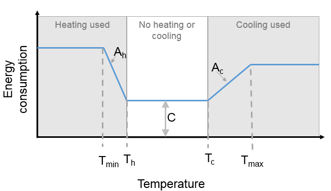
An alternative temperature response function can be used to override the
built-in values. This uses 7 parameters, illustrated below:
Fig. 14.8 Parameters used for the temperature response function
Tc: Temperature above which air conditioning is used [°C]
Th: Temperature below which heating is used [°C]
Ac: Coefficient relating temperature above Tc to energy consumption
Ah: Coefficient relating temperature below Th to energy consumption
c: Constant that sets minimum value
Tmin: Temperature below which energy use from heating stops varying
[°C]
Tmax: Temperature above which energy use from cooling stops varying
[°C]
Despite the direction of the slopes, Ah and Ac are both positive
coefficients that act on the absolute difference between T and Th or Tc
(respectively).
To activate the custom response function, the parameters must be
specified in the parameters file.
The LQF parameters file contains public holidays and numeric values used
in calculations. The table below describes the entries in each
parameters file.
14.3.8.1.2. User-defined temperature response section
To override the built-in temperature response function, the following
section must be added to the parameters file (arbitrary values are used
here as examples)
The data sources file manages the library of shapefiles and temporal
profile files used by the model. It is divided into a number of sections
(described below).
The shapefile that defines the model output areas to be used: all input
data are disaggregated into these spatial units, and the model results
are shown using them. In the simplest case, the same shapefile is used
for both outputAreas and Residential population (see below).
There are three entries:
Parameter
Description
Shapefile
Location of the shapefile on the local machine
epsgCode
EPSG code (numeric) of the shapefile coordinate reference system
featureIds
Column that contains a unique identifier for each output area (optional: order of the output areas in the file is used if empty). This is used for cross-referencing and is shown in the model outputs.
Nation-level population, vehicle registrations, energy consumption and
socio-economic data for multiple years are stored in a Spatialite
database file. The location of this file is specified in the data
sources file as follows:
Note: The population must appear under the attribute “Pop” in
the residential shapefile.
Note that a “startDate” and “epsgCode” must be specified for each
shapefile. Providing the incorrect EPSG code will result in incorrect or
zero heat fluxes being modelled because the mis-projected model areas
never overlap.
14.3.8.2.4. Temporal data: Metabolism, energy use and transportation temporal profiles
Daily mean temperature (in the local time zone of the location being
studied) is a required input. Data can be provided for multiple years
using a comma-separated list of files.
14.3.8.2.4.2. Energy consumption and traffic flow profiles (optional)
The LQF database contains default diurnal profiles for traffic and
building energy consumption, and this varies if the study area overlaps
countries with different profiles. These profiles are overridden if
user-specified data are supplied instead, and the user-specified values
are applied to the entire study area.
An example that provides all three temporal data sources is shown below,
and two years of data are provided for air temperature.
&temporal
! Mean daily air temperature data
dailyTemperature = 'C:\LQF\dailyT_2013.csv', 'C:\LQF\dailyT_2014.csv'
! Diurnal profiles
! Omit entries to use default LQF database values
diurnEnergy = 'C:\LQF\buildingProfiles.csv'
diurnTraffic = 'C:\LQF\transportProfiles.csv'
/
14.3.8.2.4.3. Using multiple temporal profile files
As with shapefiles, multiple temporal profile files can be loaded into
the model to capture different periods of time. All of the data is
combined into a single file inside the model, provided that none of the
periods described within the files clash.
A complete data sources file appears as follows. Note that two data
files are specified for the daily temperature data so that a longer time
series can be modelled.
! ### Model output polygons
&outputAreas
shapefile = 'C:\LQF\population.shp'
epsgCode = 32631
featureIds = 'ID' ! The attribute to use as a unique ID for each areas (optional; for cross-referencing)
/
! ### Residential population data for the city being studied
! Must contain total population in each area under the attribute \ “Pop”
&residentialPop
shapefiles = 'C:\LQF\population.shp'
startDates = '2014-01-01'
epsgCodes = 32631
featureIds = 'ID'
/
&database
   path = 'C:\LQF\InternationalDatabase.sqlite'
/
&temporal
! Air temperature each day for a year
dailyTemperature = 'C:\LQF\temp_2013.csv', 'C:\LQF\temp_2014.csv'
! Provide file(s) for building energy consumption and/or traffic flow diurnal cycles
! Omit entries to use default LQF database values
diurnEnergy = 'C:\LQF\buildingProfiles.csv'
diurnTraffic = 'C:\LQF\transportProfiles.csv'
/
Sometimes, a valid time zone in the Parameters or temporal input files
will be rejected by the model, resulting in a “Time zone problem” error
message.
This is usually fixed by upgrading the Python time zone library. In
Windows:
An unresolved bug causes QGIS 2.18.x to crash and quit immediately after
the “preparing input data using data sources” has finished. After
restarting QGIS, the model run can be resumed by
Using the same parameters and data sources files
Setting a new output folder
Rather than processing the input data again, selecting the prepared
input data from the old output folder.
Run the model as normal
This allows the preparation step to be skipped, making use of the
results from last time round.
14.3.10. Appendix A: Converting a population raster to a vector shapefile using QGIS
Global population datasets are generally available as raster files, but
LQF requires a set of population counts as vector polygons. This guide
explains how to convert a raster dataset to a set of polygons for use in
LQF. Examples are shown using a Greater London population count dataset
at 250m resolution.
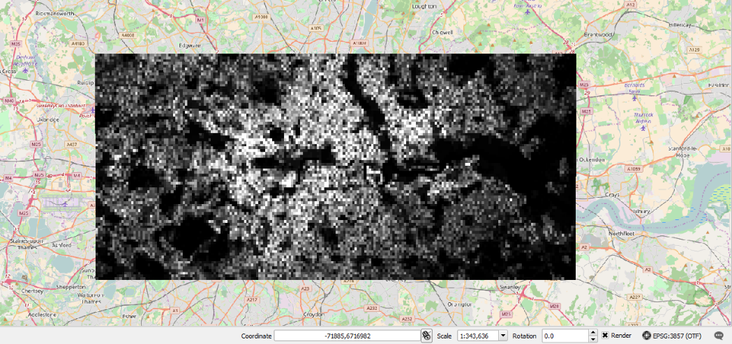
Load the raster file into QGIS
Fig. 14.9 Population raster over central London (100 meter resolution)
Rename the layer to “Pop” (this saves time later)
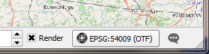
Make sure the project coordinate reference system (CRS) is the same
as for the raster. To change it, click the label and choose the
correct CRS from the list:
Fig. 14.10 Coordinate reference system (CRS) information in QGIS
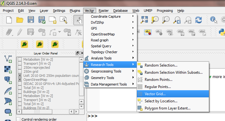
Create a vector grid aligned to the raster:
Vector -> Research Tools -> Vector Grid
Fig. 14.11 Location of vector grid tool in QGIS 2.18
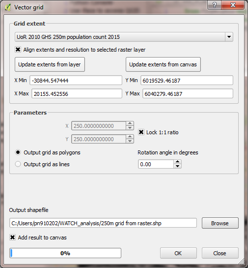
Click Align extends and resolution to the selected raster
layer (unless you want to choose the grid parameters
manually to extract a subset of the raster)
Click Update extents from layer to fill in the text boxes
If this option is not available, you will need to get the
resolution of the raster layer by inspecting its metadata
(right click the layer > Properties > Metadata > Pixel
size)
In Parameters:
Check Output grid as polygons
Choose where to save the resulting shapefile containing the
grid
Check Add results to canvas so the grid can be used
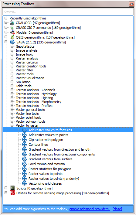
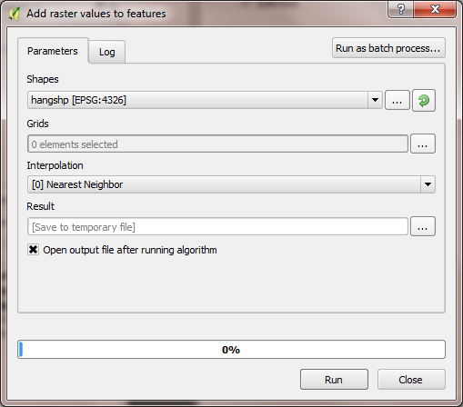
The raster values must now be extracted from the raster layer into
the vector grid. Use the “Add raster values to features” tool from
Processing > Toolbox > SAGA > Vector to raster:
Grids: Press “…” and select the “Pop” raster layer
Interpolation: Nearest neighbour (selects the nearest raster
data point)
Result: The location of a new shapefile that contains the
vector grid and the population in each cell
Press “Run”. The resulting shapefile will be added to the layers.
It contains a “Pop” column for the population
Use this shapefile as the residential population in LQF (in the
Data sources file)
14.3.11. Appendix B: Gathering information about shapefiles for QF modelling
LQF and GQF usually need two pieces of information from within a
shapefile. This section explains how to find that information:
The EPSG code, which defines the coordinate reference system. This is
needed so the model can convert between positions and units of
measurement.
Feature ID field: An attribute within the output areas file that
contains a unique identifier for each output area. This allows the
model to cross-reference between areas.
Firstly, open QGIS and load the griddedResidentialPopulation.shp file by
dragging it into the map area (canvas). An opaque grid should appear.
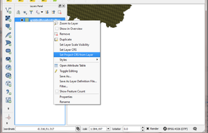
In the Layers panel, right-click “griddedResidentialPopulation” and
choose “Set project CRS from Layer”.
Fig. 14.15 Location of “Set project CRS from Layer”
The project CRS code in the bottom right-hand corner of the QGIS window will
then change to match that of the output areas file. Use the numeric part
of this to fill in the EPSGcode: entry of the data sources file:
Fig. 14.16 Coordinate reference system (CRS) information in QGIS
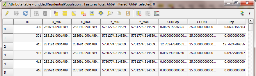
Right-click the layer again, and choose “Open Attribute Table”. The
table that appears contains one row for every output area in the file,
and one attribute for each column.
Fig. 14.17 An attribute table of a vector layer in QGIS
In this case, the column with a unique value for every output area is
called “ID”. Use this name in the DataSources file.