Note
Need help? Please let us know in the UMEP Community.
3.23. Urban Morphology: Source Area (Point)
- Contributors
Name
Institution
Christoph Kent
Reading
Fredrik Lindberg
Gothenburg
Brian Offerle
previously Indiana University; FluxSense AB
- Introduction
The Source Area or Footprint Model plugin calculates various morphometric parameters based on digital surface models and source area calculations. Footprint models can be used to determine the likely position and influence of the surface area which is contributing to a turbulent flux measurement at a specific point in time and space with imposed boundary conditions (e.g. meteorological conditions, sources/sinks of passive scalars or surface characteristics). The principle of footprint models is that the measured flux is the integral of all contributing surface elements, with a ‘footprint function’ describing the relative fractional contribution of a discretisized area.
Two footprint models exist in UMEP: (i) the Kormann and Meixner (2001) analytical footprint model; (ii) Kljun et al. (2015).
The mathematical basis of Kormann and Meixner (2001) includes a stationary gradient diffusion formulation, height independent cross-wind dispersion, power law profiles of mean wind velocity and eddy diffusivity and a power law solution of the two-dimensional advection-diffusion equation. The final solution of the footprint function is calculated by fitting the power laws (mean wind and eddy diffusivity) to Monin-Obukhov similarity profiles. As with all models, the limitations should be appreciated, which include (but are not limited to) assumptions of Monin-Obukhov similarity theory, the use of power law profiles, assumptions of horizontally homogeneous flow and assumptions of stationarity during the meteorological or scalar variable input period (i.e. their averaging period; typically 30 – 60 minutes).
Kljun et al. (2015) is a two-dimensional parameterisation for flux-footprint prediction which builds upon the footprint parameterisation of Kljun et al. (2004b) by providing the width and shape of footprint estimates, as well as explicitly considering surface roughness length. It is developed and evaluated from simulations of the backward Lagrangian stochastic particle dispersion model LPDM-B (Kljun et al., 2002) and demonstrated to be appropriate for a wide range of boundary layer conditions and measurement heights. It can therefore provide footprint estimates for a wide range of real-case applications.
When using pre-determined values of zd and z0, the horizontal wind speed is calculated internally to the respective source area models. This ensures the boundary layer equations used within the models are internally consistent.
A ground and 3D object DSM and a DEM should be used as input data. In addition if vegetation heights above ground level (i.e. trees and bushes) are available (CDSM) this can also be used. However, a CDSM need not be used and it is also possible to only use a 3D object DSM with no ground heights.
Note that the source area calculations are for one iteration. For the determination of roughness parameters, several iterations are recommended until the values converge (see Kent et al. 2017a).
- Dialog box
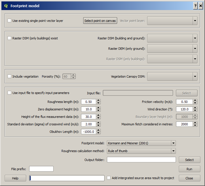
Fig. 3.52 The dialog for the Source Area (Point) calculator
- Dialog sections
upper
Select a point on the map canvas by either clicking at a location or by selecting an existing point from a point vector layer.
middle upper
Select if only buildings or both buildings and ground heights are available.
Specify the input data for buildings and ground.
middle upper 2
Select if vegetation heights are available.
Specify the input data for buildings and ground.
Specify porosity (%) of vegetation (0% is impermeable, 100 % is fully porous)
middle lower
Select input parameters to source area model: specify if a file is used, or values from the dialog box.
lower
Specify output options and run calculations.
- Select Point on Canvas
To create a point for where the calculations will take place. When you click the button, the plugin will be disabled until you have clicked the map canvas.
- Use Existing Single Point Vector Layer:
Select if you want to use a point from a vector layer that already exists and is loaded in the QGIS-project. The Vector point layer dropdown list will be enabled and include all point vector layer available.
- Raster DSM (only Building) Exist:
Select if a 3D-object DSM without ground heights is available. 3D objects (e.g. buildings) should be metres above ground.
- Raster DSM (3D Objects and Ground):
A raster DSM (e.g. geoTIFF) consisting of ground and e.g. building height (metres above sea level).
- Raster DEM (only Ground):
A DEM (e.g. geoTIFF) consisting of pixels with ground heights (metres above sea level).
- Vegetation Canopy DSM:
A CDSM (e.g. geoTIFF) consisting of pixels with vegetation heights above ground. Pixels where no objects are present should be set to zero.
- Use Input File on Specify Input Parameters:
An input text file (.txt or .csv) containing the required inputs to the model (see below) with associated time stamps. For example:
iy id it imin z_0_input z_d_input z_m_input sigv Obukhov ustar dir h por
2014 1 0 0 1.1671 8.1697 50.3 1.4805 -5457.9644 0.8460 193.8650 1000.0000 60.0000
2014 1 0 30 1.4007 9.8050 50.3 0.9616 1081.7260 0.5046 185.5874 1000.0000 60.0000
2014 1 1 0 1.3738 9.6168 50.3 0.9870 854.9901 0.4849 189.0444 1000.0000 60.0000
2014 1 1 30 1.2768 9.3872 50.3 1.2345 1002.2290 0.5876 202.3300 1000.0000 60.0000

[Header: year, day of year, hour, minutes of averaging period, roughness length for
momentum,zero plane displacement height for momentum, measurement height of sensor,
standard deviation of lateral wind,Obukhov length, friction velocity, wind direction,
boundary layer height, vegetation porosity].
Note In this example, the measurement height of the sensor (z_m_input) is 50.3
- Conditions for analysis
Parameter/Variable
Defintion
Roughness Length for Momentum
First order estimation of roughness length for momentum (z0) for this wind direction [m].
Zero Displacement Height for Momentum
First order estimation of the zero-plane displacement height for momentum (zd) for this wind direction. [m].
Measurement Height
Height of sensor above ground level [m].
Standard Deviation (sigma) of Cross Wind
Standard deviation of the wind in the y direction (lateral wind) [m s-1].
Obukhov Length
Indication of atmospheric stability for use in Monin-Obukhov similarity theory [m].
Friction Velocity
Shear stress represented in units of velocity for non-dimensional scaling [m s-1].
Wind Direction
Prevailing wind direction during averaging period [degrees].
Boundary layer height
Height of planetary boundary layer during averaging period [m].
Vegetation porosity
Aerodynamic porosity of vegetation, 0% is impermeable, 100 % is fully porous [%].
Maximum Fetch Considered in metres
The furthest distance upwind considered in the calculation of the footprint function [m].
- Footprint model
Specify the footprint model to use: Kormann and Meixner (2001) or Kljun et al. (2015)
- Roughness Calculation Method
Here, options to choose methods for roughness calculations regarding zero displacement height (zd) and roughness length (z0) are available.
RT
Rule of thumb (c.f. Grimmond and Oke 1998)
Rau
Raupach (1994)
Bot
Bottema (1998)
Mac
MacDonald et al. (1998)
Mho
Millward-Hopkins et al. (2011)
Kan
Kanda et al. (2013)
- File Prefix
A prefix that will be included in the beginning of the output files.
- Output Folder
A specified folder where result will be saved.
- Run
Starts the calculations.
- Close
Closes the plugin.
- Output:
Two different outputs are generated:
A raster grid which represents the fractional contribution of each pixel in the array to turbulent fluxes measured at the sensor (i.e. the footprint function). Each pixel of this grid will be of the same order to the input grid. Because the user can determine the maximum fetch extent that is considered, each pixel in the footprint function is weighted as a percentage of the pixel of maximum contribution. If the footprint model is set to run for more than one time period (i.e. integrated over time), the footprint functions are summed and weighted as a percentage of the pixel of maximum contribution.
A text file which specifies the time dimensions of measurements, the initial aerodynamic and meteorological parameters which were input to the model and finally the weighted geometry in the footprint and thus the newly calculated roughness length (z0) and displacement height (zd) according to the user specified method. This is of the form:
“iy id it imin z_0_input z_d_input z_m_input sigv Obukhov
 ustar dir fai pai zH zMax zSdev zd z0”

 [Header: year, day of year, hour, minutes of averaging period,
  roughness length for momentum, zero plane displacement height
  for momentum, measurement height of sensor, standard deviation
  of lateral wind, Obukhov length, friction velocity, wind direction,
  building frontal area weighted according to footprint function,
  building plan area weighted according to footprint, average height
  of buildings weighted according to footprint, maximum building height,
  standard deviation of building heights, footprint specific displacement
  height for specified method, footprint specific roughness length for
  specified method]
- Remarks
All DSMs need to have the same extent and pixel size.
Make certain that have set the projection correctly
After you haved opened the the GeoTiff files (in a new project), right click on the layer name. Set Project CRS from this layer. Now you are ready to start adding the source areas to the image.
- How to Cite
Kent et al. (2017a) unless you are including the impact of vegetation in the roughness calculations then your should cite Kent et al. (2017b).
Kent CW, CSB Grimmond, J Barlow, D Gatey, S Kotthaus, F Lindberg, CH Halios 2017: Evaluation of urban local-scale aerodynamic parameters: implications for the vertical profile of wind and source areas Boundary Layer Meteorology 164 183–213 doi: [10.1007/s10546-017-0248-z https://link.springer.com/article/10.1007/s10546-017-0248-z]
Kent CW, S Grimmond, D Gatey Aerodynamic roughness parameters in cities: inclusion of vegetation Journal of Wind Engineering & Industrial Aerodynamics http://dx.doi.org/10.1016/j.jweia.2017.07.016
- References
- Footprint Model
Kormann R and Meixner FX (2001) An analytical footprint model for non-neutral stratification. Bound-Layer Meteorol, 99, 207-224.
Kljun N, Calanca P, Rotach MW, Schmid HP (2015) A simple two-dimensional parameterisation for Flux Footprint Prediction (FFP). Geoscientific Model Development.8(11):3695-713.
- Roughness Calculations
Bottema M and Mestayer PG (1997) Urban roughness mapping–validation techniques and some first results. J Wind Eng Ind Aerodyn, 74, 163-173.
Grimmond CSB and Oke TR (1999) Aerodynamic properties of urban areas derived from analysis of surface form. J Appl Meteorol, 38, 1262-1292.
Kanda M, Inagaki A, Miyamoto T, Gryschka M and Raasch S (2013) A new aerodynamic parametrization for real urban surfaces. Bound-Layer Meteorol, 148, 357-377.
Macdonald R, Griffiths R and Hall D (1998) An improved method for the estimation of surface roughness of obstacle arrays. Atmos Environ, 32, 1857-1864.
Millward-Hopkins J, Tomlin A, Ma L, Ingham D and Pourkashanian M (2011) Estimating aerodynamic parameters of urban-like surfaces with heterogeneous building heights. Bound-Layer Meteorol, 141, 443-465.
Raupach M (1994) Simplified expressions for vegetation roughness length and zero-plane displacement as functions of canopy height and area index. Bound-Layer Meteorol, 71, 211-216.