Note
Need help? Please let us know in the UMEP Community.
12.4. GQF Manual
12.4.1. Overview
GEF provides a method to calculate the anthropogenic heat flux. It uses energy consumption, traffic and population data recorded within a city to produce estimates of the anthropogenic heat flux from buildings, transport and human metabolism at 30 minute intervals, using the highest possible spatial scale.
Spatial resolution is maximised by attributing annual industrial and domestic energy consumption (available at coarse spatial scales) to finer scales based on working and residential populations
The best available traffic and road network maps are used to attribute traffic, and therefore the heat released by burning fuel, to each spatial unit. This can be further increased based on high-resolution land cover fraction data.
Temporal resolution is maximised by applying empirically measured diurnal, day-of-week and seasonal variations to the data.
Latent, sensible and/or wastewater components of QF can be calculated.
12.4.1.1. Workflow to model QF
Select parameters and data sources files
Select output path: This contains model outputs, logs and any pre-processed data that is produced
Perform pre-processing of the data or select existing pre-processed data: This is a time-consuming step but need only to be performed once for a set of input data.
Optionally: Specify land cover fractions at high spatial resolution: Allows the spatial resolution of the modelled outputs to be enhanced
Run the model: Executes the model for the chosen date range and QF components.
Visualise outputs: A simple tool is provided to generate maps and time series from the model outputs.
12.4.2. Main user interface
The main user interface allows the user to select the temporal extent and configuration files for the model. Since the model contains many configuration options and parameters, these are stored in two files that must be managed by the user and are chosen at run time.
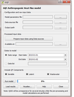
Fig. 12.18 GQF main dialogue box
Setting up and running GQF
GQF requires spatial and temporal information describing the population, energy consumption and transport in the study area. Before QF can be calculated for each part of the study area, the energy use and road network data must be disaggregated to match the chosen output areas. They are then temporally disaggregated to 30 minute resolution based on template diurnal cycles and scaling data that reflects the time of year. At the end of this process, the data are ready for use in QF calculations. GQF main dialogue box
Specify model configuration files and output path:
GQF needs configuration files that specify the spatial and temporal information to model QF:
Model parameters file: Fortran-90 namelist file containing numerical parameters required in model calculations
Data sources file: Fortran-90 namelist file that contains the locations of spatial and temporal input files used by the model
Output Path: Directory into which Model outputs and associated data will be stored. Any existing files will be overwritten.
Process input data
This step disaggregates the input data specified by the Data Sources file so that they all use the same spatial units.
The disaggregated data files are saved in the /DownscaledData/ subfolder of the chosen model output directory and can be inspected if required. This step can take up to several hours for large grids (thousands of cells), and QGIS will not respond to input while this process is going on.
If processed input data already exists elsewhere it can be used instead by specifying the path using the Available at: box. The processed files are copied to the /DownscaledData/ subfolder of the chosen model output directory. This removes the need for repeated disaggregation of the same data.
Choose temporal domain:
Dates to model (outputs are produced at 60-minute intervals). Either:
Date range: The first and final dates are specified and the whole period is simulated.
Date list: A comma-separated list of dates in YYYY-mm-dd format (e.g. 2015-01-02, 2016-03-05, 2014-05-03) is provided. These dates are simulated in their entirety.
Run model and visualise results:
The Run Model button executes the model, which applies the temporal disaggregations and calculates QF components in each output area. This takes up to several hours for high resolution or long study periods. During this time QGIS will not respond to input.
Results are visualised using the Visualise… button
Previous model results are retrieved using the Load Results button, which allows a previous model output folder to be selected.
Visualising output A simple visualisation tool accompanies the model, which produces maps and time series plots of the most recent run by default.
The results of previous runs can also be visualised without re-running the model: Select the relevant output directory and Data Sources file are chosen in the GQF UI before pressing the “Visualise” button. GQF results visualisation dialogue box
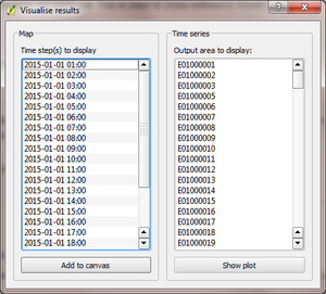
Fig. 12.19 GQF results visualisation dialogue box
Time series plots
One plot per output area is produced for all of the time steps present in the model output directory, showing the three QF components on separate axes. To plot a time series, select the output area of interest and click the “Show” button.
Maps
One map per QF component and time step is produced, coloured on a logarithmic scale according to the QF value in each output area. The map is updated in the main QGIS window each time a different QF component or time step is selected.
12.4.3. Model outputs
Model outputs are stored in the /ModelOutput/ subdirectory of the selected model output directory. A separate data file is produced for each time step of the model run. Each file contains a column per heat flux component and a row for each spatial feature.
Output files are timestamped with the patternGQFYYYYmmdd_HH-MM.csv, with times stated in UTC.
YYYY: 4-digit year
mm: 2-digit month
dd: 2-digit day of month
HH: 2-digit hour (00 to 23)
MM: 2-digit minute
The first model output is labelled 00:30 UTC and covers the period 00:00-00:30 UTC.
Each data file is in comma-separated value (CSV) format
12.4.4. Synthesised shapefiles
If pre-processing of the input data has taken place, the Disaggregated energy, transport and population shapefiles are stored in the /DownscaledData/ subdirectory of the model outputs, with filenames that reflect the time period they represent. This folder can be used as the source of processed input data in the future to save time, provided that the data sources file have not changed.
If previously processed input data are being used, the /DownscaledData/ subdirectory remains empty.
12.4.5. Logs
Several log files are saved in the /Logs/ subdirectory. The logs are intended to help interpretation of model outputs by providing a traceable history of why a particular spatial or temporal disaggregation value was looked up.
The steps taken to disaggregate spatial data, including which attributes were involved
The day of week and the time of day that was returned from each diurnal and annual profile data source when it was queried with a particular model time step.
12.4.6. Configuration files
The Parameters and Data Sources file are copied to the /ConfigFiles/ subdirectory of the model output directory for future reference.
12.4.7. Input data
Input data consists of spatial and temporal information, a lookup table for vehicle fuel efficiency and (optionally) land use cover data to further enhance the spatial resolution of the model output.
Spatial information:
Residential (evening) and work day (daytime) absolute population
District-scale domestic and industrial energy consumption [kWh/year]
Road network topography and associated traffic flows
Temporal information (provided via CSV files):
Template diurnal cycles for energy consumption, traffic flow and human activity
Variations of these cycles for different days of week
Variations of the above at different times of year.
12.4.7.1. Spatial data
This section lists the spatial data (provided via ESRI shapefiles) required by the model. Each shapefile must contain:
Polygons representing each spatial area (except for Transport)
An attribute that contains a unique identifier for each polygon. This is needed for objective cross-referencing of data within the model.
12.4.7.1.1. Population data
Population data [number of people per spatial unit] is used by the model in two ways:
Calculating metabolic emissions in different areas
Attributing domestic and industrial energy use at a finer spatial scale.
Two types of population are needed:
Residential/evening population: The population residing in each area
Workday/daytime population: The population at work or home during the daytime in each area
Since population data are key to the model method, it is important to use the finest available spatial scale.
The model must output results for a consistent set of spatial units, so the populations are assigned to the model output areas based on how much each spatial unit of population is intersected each output area. It is recommended that a population shapefile is chosen as the output areas.
12.4.7.1.2. Energy consumption data
The total annual energy consumption [kWh/year] must be provided five sub-sectors
Industrial electricity
Industrial gas
Domestic electricity
Domestic gas
Domestic “Economy 7”: an electrical supply with a distinct diurnal pattern (may be set to zero in the data sources file if not available)
This data is used to calculate heat emissions from residential and industrial buildings, and is generally available in coarse spatial units. Residential and workday population data are therefore used to spatially disaggregate it into the model output areas.
12.4.7.1.3. Transportation data
A comprehensive road network shapefile is required.
Minimum: vector line for each segment of the road network, together with the type of road each segment represents.
Four road classes are assumed in the model:
Motorway |
Purpose-built highways |
Primary road |
Major thoroughfares |
Secondary road |
Thoroughfares with less traffic |
Other |
Any other road segments: Assumed to have minor traffic flow |
The naming convention used in the shapefile must be defined in the transport section of the Data sources file for the first three.
Diesel and petrol consumption are calculated for seven vehicle types indicated using any segment-specific traffic flow and speed data available. This is combined with fuel consumption data. The vehicle types are:
Name in model |
Description |
|---|---|
Motorcycle |
Motorcycles |
Taxi |
Taxis |
Bus |
Buses and coaches |
Artic |
Articulated trucks |
Rigid |
Rigid body trucks |
LGV |
Light Goods Vehicle |
Car |
Ordinary cars |
Fuel consumption for a given vehicle type on a particular road segment [g/day] is estimated by multiplying:
Speed, fuel and vehicle-dependent consumption rates [g/km] from the COPERT-II database, which lists consumption for different vehicle types under different Euro-class regimes that apply to vehicles manufactured after a particular date.
Length of the road segment [km]
Vehicle type and fuel-dependent average daily total (AADT) number of vehicles passing over the road segment.
Each road segment in the shapefile would ideally be accompanied by a speed for the segment and an AADT for each vehicle type that is further broken down into diesel and petrol components for cars and LGVs. It is not always possible to obtain some or even any of these, so default representative values must also be specified in the `model parameters file Parameters_file:
AADT |
A representative AADT associated with each road class |
Road fleet fraction |
Contribution of different vehicle types to the total traffic on each road classification. |
Fuel fraction |
Fraction of each vehicle type powered by diesel and petrol |
Speed |
Typical speed of traffic on each road classification |
The use of the default parameters depends upon the available information in the shapefile. This relations are summarised below: when parameters are used if certain information are (green) or are not (red) available.
Available in shapefile
Total AADT |
AADT by vehicle |
AADT by vehicle & fuel |
Speed |
|---|---|---|---|
X |
X |
X |
X |
/ |
X |
X |
X |
/ |
/ |
X |
X |
/ |
/ |
/ |
X |
X |
X |
X |
/ |
X |
X |
X |
/ |
/ |
X |
X |
/ |
/ |
/ |
X |
/ |
/ |
/ |
/ |
/ |
Looked up from parameters
AADT |
Fuel fraction |
Fleet fraction |
Speed |
|---|---|---|---|
/ |
/ |
/ |
/ |
X |
/ |
/ |
/ |
X |
/ |
X |
/ |
X |
X |
X |
/ |
/ |
/ |
/ |
X |
/ |
/ |
/ |
X |
X |
/ |
/ |
X |
X |
/ |
X |
X |
X |
X |
X |
X |
The fuel consumption that a segment contributes to a model output area (OA) is calculated by determining the proportion of the segment that intersects the OA and multiplying the total segment consumption by this. Total fuel consumption inside an output area is calculated by summing over all the segments that intersect it. This yields a new shapefile in which each output area is associated with a daily petrol and diesel consumption.
Daily fuel consumption in an OA is converted to mean heat flux [W m-2] using the heat of combustion [J kg-1], number of seconds in a day and the area of the OA [m-2]. This is disaggregated to half-hour time steps using empirical diurnal cycle data for each day of the week.
12.4.7.1.4. Time indexing of spatial data
A series of shapefiles, each associated with a different start date, can be loaded into the model to capture the time evolution of energy use, transport or population. The following example describes how such a series is treated by the model implementation:
Two shapefiles are provided for population. The first is correct as of 2015-01-01, and the second is correct as of 2016-01-01. The model is set to calculate QF from 2014 to 2017 continuously:
Model time steps representing dates before 2015-01-01 use the earliest available shapefile (2015-01-01).
Model time steps on/after 2015-01-01 but before 2016-01-01 use the 2015-01-01 shapefile
Model time steps on/after 2016-01-01 use the 2016-01-01 shapefile. No transition is assumed between the shapefiles.
Since energy consumption data is disaggregated to finer spatial units based on population, the energy consumption on/before 2015-12-31 is disaggregated using the 2015-01-01 population data, while energy consumption associated with 2016-01-01 or later is disaggregated using the 2016-01-01 population data.
12.4.7.2. Temporal files required by GQF
Overview
Four temporal profile files (summarised below) contain information about half-hourly, daily and seasonal variations in traffic, metabolic activity and energy use. These allow the annualised data provided by the shapefiles to be temporally disaggreated into time series.
Each file must contain:
A time series of values at 30 minute intervals, binned to the right hand side. The first entry of every file represents the period 00:00-00:30 and is labelled 00:30.
Values for every part of every year mentioned in the file. Gaps are not allowed.
The time zone represented by the file (“UTC” or of the style “Europe/London”). If “UTC” is specified, then values must be explicitly provided for each daylight savings regime to capture shifts in human behaviour. Note that the model outputs are always UTC, with the necessary conversion taking place in the software.
The start and end dates of the period represented by the data. This allows seasonality to be captured.
QF component |
File description(s) |
Size of file |
|---|---|---|
Metabolism |
Diurnal cycles of metabolic activity for each day of week and each season |
48 half-hours * 7 days * N seasons |
Transport |
Traffic flows for each vehicle type during each day of the week |
336 half-hours (=48 * 7) * 7 vehicle types |
Building energy |
Seasonal variations: Daily total gas and electricity consumption variation (one file for electricity and gas) |
365 (or 366) days * 2 fuel types |
Diurnal variations: Template cycles for weekdays, Saturdays and Sundays for each season (separate file for each fuel) |
48 half-hours * 3 day types * N seasons |
Ideally these files contain data taken from the period being modelled, but this is not always practical. In this case, temporal profile data from the most recent available year is looked up for the same day of week (taking into account public holidays), season and daylight savings regime if applicable. Different variants are used for traffic, energy and metabolism, and each of these is described below.
12.4.7.2.1. Details of temporal files
12.4.7.2.1.1. Traffic flow profiles
A template week of traffic variations at 30 min intervals (336 entries, 48 * 7) beginning on Monday must be specified for each vehicle type, so that day of week effects are captured.
An example is shown below. The first header line must be exactly as shown because it specifies the vehicle types used in the model. Each file may contain only one set of values. Subsequent periods or years must be stored in separate files.
TransportType |
motorcycles |
taxis |
cars |
Buses |
LGVs |
rigids |
artics |
|---|---|---|---|---|---|---|---|
StartDate |
2016-01-01 |
||||||
EndDate |
2016-12-31 |
||||||
Timezone |
Europe/London |
||||||
00:30 |
0.237 |
1.125 |
0.398 |
0.594 |
0.198 |
0.435 |
0.436 |
01:00 |
0.178 |
1.003 |
0.312 |
0.433 |
0.172 |
0.393 |
0.4 |
01:30 |
0.12 |
0.881 |
0.226 |
0.272 |
0.146 |
0.352 |
0.365 |
02:00 |
0.093 |
0.647 |
0.192 |
0.234 |
0.138 |
0.378 |
0.378 |
02:30 |
0.066 |
0.412 |
0.159 |
0.197 |
0.13 |
0.404 |
0.39 |
03:00 |
0.065 |
0.349 |
0.147 |
0.189 |
0.148 |
0.355 |
0.366 |
03:30 |
0.063 |
0.286 |
0.135 |
0.18 |
0.167 |
0.306 |
0.342 |
04:00 |
0.086 |
0.276 |
0.149 |
0.204 |
0.215 |
0.413 |
0.427 |
04:30 |
0.109 |
0.267 |
0.163 |
0.229 |
0.262 |
0.52 |
0.511 |
05:00 |
0.199 |
0.343 |
0.226 |
0.367 |
0.341 |
0.7 |
0.664 |
05:30 |
0.288 |
0.419 |
0.288 |
0.505 |
0.42 |
0.88 |
0.817 |
06:00 |
0.699 |
0.565 |
0.54 |
0.721 |
0.934 |
1.195 |
1.161 |
06:30 |
1.11 |
0.71 |
0.791 |
0.937 |
1.448 |
1.511 |
1.504 |
07:00 |
1.62 |
0.786 |
1.086 |
1.184 |
1.771 |
1.5 |
1.646 |
07:30 |
2.129 |
0.861 |
1.381 |
1.431 |
2.094 |
1.49 |
1.788 |
08:00 |
2.375 |
0.873 |
1.461 |
1.435 |
1.875 |
1.498 |
1.739 |
08:30 |
2.62 |
0.885 |
1.54 |
1.438 |
1.656 |
1.507 |
1.689 |
09:00 |
2.166 |
0.897 |
1.424 |
1.487 |
1.672 |
1.693 |
1.791 |
09:30 |
1.712 |
0.909 |
1.308 |
1.537 |
1.689 |
1.88 |
1.892 |
10:00 |
1.452 |
0.983 |
1.23 |
1.499 |
1.724 |
1.96 |
1.956 |
10:30 |
1.192 |
1.057 |
1.152 |
1.462 |
1.76 |
2.041 |
2.02 |
11:00 |
1.165 |
1.095 |
1.144 |
1.404 |
1.765 |
2.077 |
2.025 |
11:30 |
1.138 |
1.133 |
1.136 |
1.347 |
1.77 |
2.112 |
2.031 |
12:00 |
1.167 |
1.125 |
1.168 |
1.335 |
1.76 |
2.118 |
2.034 |
12:30 |
1.196 |
1.117 |
1.2 |
1.324 |
1.75 |
2.124 |
2.037 |
13:00 |
1.239 |
1.143 |
1.209 |
1.339 |
1.748 |
2.072 |
1.988 |
13:30 |
1.282 |
1.169 |
1.219 |
1.354 |
1.746 |
2.021 |
1.94 |
14:00 |
1.292 |
1.281 |
1.231 |
1.392 |
1.775 |
1.97 |
1.862 |
14:30 |
1.302 |
1.393 |
1.244 |
1.43 |
1.804 |
1.919 |
1.784 |
15:00 |
1.375 |
1.321 |
1.31 |
1.454 |
1.838 |
1.853 |
1.678 |
15:30 |
1.447 |
1.248 |
1.376 |
1.477 |
1.872 |
1.788 |
1.572 |
16:00 |
1.671 |
1.337 |
1.448 |
1.504 |
1.887 |
1.665 |
1.468 |
16:30 |
1.894 |
1.425 |
1.521 |
1.531 |
1.902 |
1.542 |
1.363 |
17:00 |
2.237 |
1.447 |
1.606 |
1.47 |
1.714 |
1.419 |
1.241 |
17:30 |
2.579 |
1.469 |
1.691 |
1.41 |
1.525 |
1.296 |
1.119 |
18:00 |
2.518 |
1.414 |
1.647 |
1.377 |
1.314 |
1.214 |
1.038 |
18:30 |
2.458 |
1.36 |
1.604 |
1.343 |
1.103 |
1.132 |
0.956 |
19:00 |
2.086 |
1.394 |
1.54 |
1.33 |
0.973 |
0.799 |
0.733 |
19:30 |
1.715 |
1.429 |
1.476 |
1.318 |
0.843 |
0.466 |
0.511 |
20:00 |
1.417 |
1.445 |
1.314 |
1.195 |
0.724 |
0.462 |
0.498 |
20:30 |
1.119 |
1.461 |
1.153 |
1.071 |
0.604 |
0.459 |
0.485 |
21:00 |
0.963 |
1.396 |
1.054 |
0.971 |
0.52 |
0.384 |
0.427 |
21:30 |
0.807 |
1.331 |
0.954 |
0.871 |
0.437 |
0.31 |
0.37 |
22:00 |
0.705 |
1.301 |
0.893 |
0.807 |
0.384 |
0.338 |
0.381 |
22:30 |
0.602 |
1.271 |
0.832 |
0.744 |
0.331 |
0.365 |
0.393 |
23:00 |
0.525 |
1.287 |
0.748 |
0.745 |
0.3 |
0.409 |
0.424 |
23:30 |
0.447 |
1.304 |
0.665 |
0.747 |
0.269 |
0.453 |
0.455 |
00:00 |
0.346 |
1.235 |
0.539 |
0.681 |
0.237 |
0.452 |
0.453 |
00:30 |
0.246 |
1.167 |
0.412 |
0.616 |
0.206 |
0.451 |
0.451 |
01:00 |
0.185 |
1.04 |
0.323 |
0.449 |
0.178 |
0.408 |
0.415 |
01:30 |
0.125 |
0.914 |
0.234 |
0.282 |
0.151 |
0.365 |
0.378 |
02:00 |
0.097 |
0.671 |
0.2 |
0.243 |
0.143 |
0.392 |
0.391 |
02:30 |
0.069 |
0.428 |
0.165 |
0.205 |
0.134 |
0.419 |
0.404 |
03:00 |
0.067 |
0.362 |
0.153 |
0.195 |
0.154 |
0.368 |
0.379 |
03:30 |
0.066 |
0.297 |
0.14 |
0.186 |
0.173 |
0.317 |
0.354 |
04:00 |
0.089 |
0.287 |
0.155 |
0.212 |
0.222 |
0.428 |
0.442 |
04:30 |
0.113 |
0.277 |
0.17 |
0.238 |
0.272 |
0.539 |
0.53 |
05:00 |
0.206 |
0.355 |
0.234 |
0.381 |
0.354 |
0.725 |
0.688 |
05:30 |
0.299 |
0.434 |
0.299 |
0.524 |
0.436 |
0.911 |
0.847 |
06:00 |
0.726 |
0.586 |
0.56 |
0.748 |
0.968 |
1.239 |
1.203 |
06:30 |
1.153 |
0.737 |
0.821 |
0.972 |
1.5 |
1.566 |
1.559 |
07:00 |
1.676 |
0.813 |
1.124 |
1.225 |
1.832 |
1.552 |
1.703 |
07:30 |
2.199 |
0.89 |
1.427 |
1.478 |
2.163 |
1.539 |
1.847 |
08:00 |
2.47 |
0.908 |
1.519 |
1.491 |
1.947 |
1.557 |
1.807 |
08:30 |
2.74 |
0.925 |
1.611 |
1.504 |
1.732 |
1.576 |
1.767 |
09:00 |
2.264 |
0.937 |
1.488 |
1.554 |
1.748 |
1.769 |
1.871 |
09:30 |
1.787 |
0.949 |
1.366 |
1.605 |
1.763 |
1.963 |
1.976 |
10:00 |
1.515 |
1.025 |
1.283 |
1.564 |
1.799 |
2.045 |
2.04 |
10:30 |
1.243 |
1.101 |
1.201 |
1.523 |
1.834 |
2.127 |
2.105 |
11:00 |
1.211 |
1.138 |
1.189 |
1.459 |
1.834 |
2.158 |
2.105 |
11:30 |
1.18 |
1.174 |
1.177 |
1.396 |
1.835 |
2.189 |
2.105 |
12:00 |
1.207 |
1.163 |
1.207 |
1.381 |
1.82 |
2.19 |
2.103 |
12:30 |
1.233 |
1.152 |
1.237 |
1.366 |
1.805 |
2.191 |
2.101 |
13:00 |
1.275 |
1.176 |
1.245 |
1.378 |
1.799 |
2.133 |
2.047 |
13:30 |
1.317 |
1.201 |
1.252 |
1.391 |
1.794 |
2.076 |
1.993 |
14:00 |
1.329 |
1.317 |
1.266 |
1.432 |
1.825 |
2.025 |
1.914 |
14:30 |
1.34 |
1.434 |
1.28 |
1.472 |
1.856 |
1.974 |
1.836 |
15:00 |
1.416 |
1.36 |
1.349 |
1.497 |
1.892 |
1.908 |
1.728 |
15:30 |
1.491 |
1.286 |
1.418 |
1.522 |
1.929 |
1.843 |
1.62 |
16:00 |
1.721 |
1.377 |
1.492 |
1.549 |
1.944 |
1.715 |
1.512 |
16:30 |
1.95 |
1.468 |
1.566 |
1.576 |
1.959 |
1.588 |
1.404 |
17:00 |
2.318 |
1.499 |
1.663 |
1.522 |
1.774 |
1.469 |
1.285 |
17:30 |
2.686 |
1.53 |
1.761 |
1.469 |
1.589 |
1.35 |
1.166 |
18:00 |
2.635 |
1.48 |
1.723 |
1.44 |
1.374 |
1.27 |
1.086 |
18:30 |
2.583 |
1.43 |
1.686 |
1.412 |
1.16 |
1.189 |
1.005 |
19:00 |
2.182 |
1.456 |
1.608 |
1.389 |
1.017 |
0.836 |
0.767 |
19:30 |
1.78 |
1.482 |
1.531 |
1.366 |
0.874 |
0.483 |
0.529 |
20:00 |
1.471 |
1.498 |
1.363 |
1.239 |
0.75 |
0.479 |
0.516 |
20:30 |
1.162 |
1.515 |
1.196 |
1.111 |
0.626 |
0.475 |
0.503 |
21:00 |
1 |
1.448 |
1.093 |
1.007 |
0.539 |
0.398 |
0.443 |
21:30 |
0.838 |
1.381 |
0.989 |
0.903 |
0.452 |
0.322 |
0.383 |
22:00 |
0.732 |
1.349 |
0.926 |
0.837 |
0.398 |
0.35 |
0.395 |
22:30 |
0.625 |
1.318 |
0.863 |
0.772 |
0.343 |
0.378 |
0.407 |
23:00 |
0.545 |
1.335 |
0.776 |
0.773 |
0.311 |
0.424 |
0.439 |
23:30 |
0.464 |
1.352 |
0.69 |
0.774 |
0.279 |
0.47 |
0.471 |
00:00 |
0.355 |
1.261 |
0.552 |
0.696 |
0.243 |
0.461 |
0.462 |
00:30 |
0.247 |
1.171 |
0.414 |
0.618 |
0.207 |
0.452 |
0.453 |
01:00 |
0.186 |
1.044 |
0.324 |
0.45 |
0.179 |
0.409 |
0.416 |
01:30 |
0.125 |
0.917 |
0.235 |
0.283 |
0.152 |
0.366 |
0.38 |
02:00 |
0.097 |
0.673 |
0.2 |
0.244 |
0.143 |
0.393 |
0.393 |
02:30 |
0.069 |
0.429 |
0.166 |
0.205 |
0.135 |
0.421 |
0.406 |
03:00 |
0.067 |
0.363 |
0.153 |
0.196 |
0.154 |
0.369 |
0.381 |
03:30 |
0.066 |
0.298 |
0.141 |
0.187 |
0.174 |
0.318 |
0.356 |
04:00 |
0.09 |
0.288 |
0.155 |
0.213 |
0.223 |
0.43 |
0.444 |
04:30 |
0.114 |
0.278 |
0.17 |
0.238 |
0.273 |
0.541 |
0.532 |
05:00 |
0.207 |
0.357 |
0.235 |
0.382 |
0.355 |
0.728 |
0.691 |
05:30 |
0.3 |
0.436 |
0.3 |
0.526 |
0.437 |
0.915 |
0.851 |
06:00 |
0.729 |
0.588 |
0.562 |
0.751 |
0.972 |
1.243 |
1.208 |
06:30 |
1.157 |
0.739 |
0.823 |
0.976 |
1.507 |
1.572 |
1.566 |
07:00 |
1.695 |
0.822 |
1.136 |
1.238 |
1.851 |
1.567 |
1.721 |
07:30 |
2.233 |
0.904 |
1.449 |
1.501 |
2.196 |
1.562 |
1.876 |
08:00 |
2.496 |
0.918 |
1.535 |
1.507 |
1.97 |
1.574 |
1.827 |
08:30 |
2.759 |
0.932 |
1.621 |
1.514 |
1.743 |
1.586 |
1.779 |
09:00 |
2.273 |
0.94 |
1.493 |
1.559 |
1.753 |
1.774 |
1.877 |
09:30 |
1.786 |
0.949 |
1.365 |
1.604 |
1.762 |
1.962 |
1.975 |
10:00 |
1.518 |
1.028 |
1.286 |
1.568 |
1.803 |
2.05 |
2.046 |
10:30 |
1.249 |
1.107 |
1.207 |
1.531 |
1.844 |
2.139 |
2.116 |
11:00 |
1.219 |
1.145 |
1.197 |
1.469 |
1.847 |
2.172 |
2.119 |
11:30 |
1.189 |
1.183 |
1.186 |
1.407 |
1.849 |
2.206 |
2.121 |
12:00 |
1.212 |
1.168 |
1.213 |
1.387 |
1.828 |
2.2 |
2.112 |
12:30 |
1.235 |
1.153 |
1.239 |
1.367 |
1.807 |
2.193 |
2.103 |
13:00 |
1.278 |
1.179 |
1.247 |
1.381 |
1.802 |
2.137 |
2.051 |
13:30 |
1.321 |
1.204 |
1.255 |
1.395 |
1.798 |
2.081 |
1.998 |
14:00 |
1.333 |
1.321 |
1.27 |
1.436 |
1.83 |
2.031 |
1.92 |
14:30 |
1.344 |
1.439 |
1.284 |
1.477 |
1.862 |
1.981 |
1.842 |
15:00 |
1.421 |
1.364 |
1.353 |
1.502 |
1.899 |
1.915 |
1.734 |
15:30 |
1.497 |
1.29 |
1.423 |
1.527 |
1.936 |
1.849 |
1.626 |
16:00 |
1.733 |
1.386 |
1.502 |
1.559 |
1.956 |
1.726 |
1.521 |
16:30 |
1.968 |
1.481 |
1.58 |
1.591 |
1.977 |
1.603 |
1.417 |
17:00 |
2.317 |
1.5 |
1.664 |
1.524 |
1.777 |
1.471 |
1.287 |
17:30 |
2.666 |
1.519 |
1.748 |
1.458 |
1.577 |
1.34 |
1.157 |
18:00 |
2.623 |
1.473 |
1.716 |
1.434 |
1.368 |
1.264 |
1.081 |
18:30 |
2.58 |
1.428 |
1.684 |
1.41 |
1.158 |
1.188 |
1.004 |
19:00 |
2.183 |
1.457 |
1.61 |
1.391 |
1.018 |
0.837 |
0.768 |
19:30 |
1.786 |
1.487 |
1.536 |
1.372 |
0.877 |
0.485 |
0.531 |
20:00 |
1.476 |
1.504 |
1.368 |
1.243 |
0.753 |
0.481 |
0.518 |
20:30 |
1.166 |
1.52 |
1.201 |
1.115 |
0.629 |
0.477 |
0.505 |
21:00 |
1.004 |
1.453 |
1.097 |
1.011 |
0.542 |
0.4 |
0.445 |
21:30 |
0.841 |
1.385 |
0.993 |
0.906 |
0.454 |
0.323 |
0.385 |
22:00 |
0.734 |
1.354 |
0.929 |
0.84 |
0.399 |
0.351 |
0.397 |
22:30 |
0.627 |
1.322 |
0.866 |
0.775 |
0.344 |
0.38 |
0.409 |
23:00 |
0.546 |
1.34 |
0.779 |
0.776 |
0.312 |
0.426 |
0.441 |
23:30 |
0.466 |
1.357 |
0.692 |
0.777 |
0.28 |
0.472 |
0.473 |
00:00 |
0.357 |
1.269 |
0.555 |
0.7 |
0.244 |
0.464 |
0.465 |
00:30 |
0.249 |
1.181 |
0.418 |
0.623 |
0.208 |
0.456 |
0.457 |
01:00 |
0.188 |
1.053 |
0.327 |
0.454 |
0.181 |
0.413 |
0.42 |
01:30 |
0.126 |
0.925 |
0.237 |
0.285 |
0.153 |
0.369 |
0.383 |
02:00 |
0.098 |
0.679 |
0.202 |
0.246 |
0.145 |
0.397 |
0.396 |
02:30 |
0.069 |
0.433 |
0.167 |
0.207 |
0.136 |
0.424 |
0.409 |
03:00 |
0.068 |
0.367 |
0.155 |
0.198 |
0.156 |
0.372 |
0.384 |
03:30 |
0.066 |
0.3 |
0.142 |
0.189 |
0.175 |
0.321 |
0.359 |
04:00 |
0.091 |
0.29 |
0.157 |
0.215 |
0.225 |
0.433 |
0.448 |
04:30 |
0.115 |
0.28 |
0.172 |
0.24 |
0.275 |
0.546 |
0.536 |
05:00 |
0.209 |
0.36 |
0.237 |
0.385 |
0.358 |
0.734 |
0.697 |
05:30 |
0.303 |
0.44 |
0.303 |
0.53 |
0.441 |
0.923 |
0.858 |
06:00 |
0.735 |
0.593 |
0.567 |
0.757 |
0.98 |
1.254 |
1.218 |
06:30 |
1.167 |
0.746 |
0.831 |
0.984 |
1.519 |
1.585 |
1.578 |
07:00 |
1.707 |
0.828 |
1.144 |
1.247 |
1.864 |
1.578 |
1.733 |
07:30 |
2.247 |
0.909 |
1.458 |
1.51 |
2.209 |
1.572 |
1.887 |
08:00 |
2.506 |
0.921 |
1.541 |
1.514 |
1.978 |
1.581 |
1.835 |
08:30 |
2.764 |
0.933 |
1.625 |
1.517 |
1.747 |
1.59 |
1.782 |
09:00 |
2.282 |
0.945 |
1.5 |
1.567 |
1.762 |
1.783 |
1.886 |
09:30 |
1.8 |
0.956 |
1.375 |
1.617 |
1.776 |
1.977 |
1.99 |
10:00 |
1.524 |
1.031 |
1.291 |
1.573 |
1.809 |
2.057 |
2.053 |
10:30 |
1.249 |
1.107 |
1.206 |
1.53 |
1.843 |
2.137 |
2.115 |
11:00 |
1.217 |
1.143 |
1.194 |
1.466 |
1.842 |
2.168 |
2.114 |
11:30 |
1.185 |
1.179 |
1.182 |
1.401 |
1.842 |
2.198 |
2.113 |
12:00 |
1.214 |
1.17 |
1.215 |
1.389 |
1.831 |
2.204 |
2.116 |
12:30 |
1.244 |
1.162 |
1.248 |
1.377 |
1.82 |
2.209 |
2.119 |
13:00 |
1.296 |
1.195 |
1.264 |
1.4 |
1.827 |
2.166 |
2.079 |
13:30 |
1.347 |
1.228 |
1.281 |
1.423 |
1.834 |
2.123 |
2.038 |
14:00 |
1.359 |
1.348 |
1.295 |
1.465 |
1.867 |
2.072 |
1.958 |
14:30 |
1.371 |
1.467 |
1.31 |
1.506 |
1.9 |
2.021 |
1.879 |
15:00 |
1.443 |
1.387 |
1.375 |
1.526 |
1.93 |
1.946 |
1.762 |
15:30 |
1.515 |
1.306 |
1.44 |
1.546 |
1.96 |
1.872 |
1.646 |
16:00 |
1.746 |
1.397 |
1.514 |
1.572 |
1.973 |
1.741 |
1.535 |
16:30 |
1.977 |
1.488 |
1.588 |
1.598 |
1.986 |
1.61 |
1.423 |
17:00 |
2.339 |
1.513 |
1.679 |
1.537 |
1.791 |
1.483 |
1.298 |
17:30 |
2.701 |
1.538 |
1.77 |
1.477 |
1.597 |
1.357 |
1.172 |
18:00 |
2.657 |
1.492 |
1.738 |
1.452 |
1.385 |
1.28 |
1.094 |
18:30 |
2.613 |
1.446 |
1.705 |
1.428 |
1.173 |
1.203 |
1.017 |
19:00 |
2.207 |
1.473 |
1.627 |
1.405 |
1.029 |
0.846 |
0.776 |
19:30 |
1.801 |
1.5 |
1.549 |
1.383 |
0.885 |
0.489 |
0.536 |
20:00 |
1.489 |
1.517 |
1.38 |
1.254 |
0.759 |
0.485 |
0.522 |
20:30 |
1.176 |
1.534 |
1.211 |
1.125 |
0.634 |
0.481 |
0.509 |
21:00 |
1.012 |
1.465 |
1.106 |
1.019 |
0.546 |
0.403 |
0.448 |
21:30 |
0.848 |
1.397 |
1.001 |
0.914 |
0.458 |
0.326 |
0.388 |
22:00 |
0.741 |
1.366 |
0.937 |
0.848 |
0.403 |
0.354 |
0.4 |
22:30 |
0.633 |
1.334 |
0.873 |
0.781 |
0.347 |
0.383 |
0.412 |
23:00 |
0.551 |
1.351 |
0.786 |
0.782 |
0.315 |
0.429 |
0.445 |
23:30 |
0.47 |
1.369 |
0.698 |
0.784 |
0.283 |
0.476 |
0.477 |
00:00 |
0.358 |
1.271 |
0.557 |
0.702 |
0.245 |
0.465 |
0.466 |
00:30 |
0.247 |
1.174 |
0.415 |
0.619 |
0.207 |
0.453 |
0.454 |
01:00 |
0.186 |
1.047 |
0.325 |
0.451 |
0.179 |
0.41 |
0.417 |
01:30 |
0.126 |
0.92 |
0.235 |
0.283 |
0.152 |
0.367 |
0.38 |
02:00 |
0.097 |
0.675 |
0.201 |
0.245 |
0.144 |
0.394 |
0.393 |
02:30 |
0.069 |
0.43 |
0.166 |
0.206 |
0.135 |
0.422 |
0.407 |
03:00 |
0.068 |
0.364 |
0.154 |
0.197 |
0.155 |
0.37 |
0.382 |
03:30 |
0.066 |
0.299 |
0.141 |
0.187 |
0.174 |
0.319 |
0.356 |
04:00 |
0.09 |
0.288 |
0.156 |
0.213 |
0.224 |
0.431 |
0.445 |
04:30 |
0.114 |
0.278 |
0.171 |
0.239 |
0.273 |
0.542 |
0.533 |
05:00 |
0.207 |
0.358 |
0.236 |
0.383 |
0.356 |
0.73 |
0.692 |
05:30 |
0.301 |
0.437 |
0.301 |
0.527 |
0.438 |
0.917 |
0.852 |
06:00 |
0.73 |
0.589 |
0.563 |
0.752 |
0.974 |
1.246 |
1.21 |
06:30 |
1.159 |
0.741 |
0.825 |
0.978 |
1.509 |
1.575 |
1.568 |
07:00 |
1.677 |
0.815 |
1.125 |
1.226 |
1.834 |
1.555 |
1.706 |
07:30 |
2.195 |
0.888 |
1.424 |
1.475 |
2.158 |
1.535 |
1.843 |
08:00 |
2.456 |
0.903 |
1.511 |
1.483 |
1.938 |
1.549 |
1.798 |
08:30 |
2.718 |
0.918 |
1.598 |
1.492 |
1.718 |
1.563 |
1.753 |
09:00 |
2.25 |
0.932 |
1.479 |
1.546 |
1.738 |
1.76 |
1.861 |
09:30 |
1.781 |
0.946 |
1.361 |
1.6 |
1.757 |
1.956 |
1.969 |
10:00 |
1.51 |
1.022 |
1.279 |
1.559 |
1.793 |
2.039 |
2.034 |
10:30 |
1.239 |
1.098 |
1.197 |
1.519 |
1.828 |
2.121 |
2.099 |
11:00 |
1.216 |
1.143 |
1.194 |
1.465 |
1.842 |
2.167 |
2.114 |
11:30 |
1.193 |
1.188 |
1.19 |
1.412 |
1.856 |
2.214 |
2.129 |
12:00 |
1.22 |
1.176 |
1.221 |
1.396 |
1.84 |
2.214 |
2.126 |
12:30 |
1.247 |
1.164 |
1.251 |
1.38 |
1.824 |
2.214 |
2.124 |
13:00 |
1.29 |
1.19 |
1.259 |
1.394 |
1.82 |
2.158 |
2.071 |
13:30 |
1.334 |
1.216 |
1.268 |
1.408 |
1.816 |
2.102 |
2.017 |
14:00 |
1.346 |
1.334 |
1.282 |
1.45 |
1.848 |
2.052 |
1.939 |
14:30 |
1.358 |
1.453 |
1.297 |
1.492 |
1.881 |
2.001 |
1.861 |
15:00 |
1.431 |
1.375 |
1.364 |
1.514 |
1.914 |
1.93 |
1.748 |
15:30 |
1.505 |
1.297 |
1.43 |
1.535 |
1.946 |
1.859 |
1.634 |
16:00 |
1.741 |
1.392 |
1.509 |
1.567 |
1.966 |
1.734 |
1.529 |
16:30 |
1.977 |
1.488 |
1.587 |
1.598 |
1.986 |
1.61 |
1.423 |
17:00 |
2.335 |
1.511 |
1.677 |
1.535 |
1.789 |
1.482 |
1.296 |
17:30 |
2.693 |
1.534 |
1.766 |
1.473 |
1.593 |
1.353 |
1.169 |
18:00 |
2.659 |
1.493 |
1.739 |
1.453 |
1.386 |
1.281 |
1.095 |
18:30 |
2.625 |
1.452 |
1.713 |
1.434 |
1.178 |
1.208 |
1.021 |
19:00 |
2.207 |
1.472 |
1.626 |
1.404 |
1.029 |
0.847 |
0.777 |
19:30 |
1.789 |
1.491 |
1.54 |
1.374 |
0.879 |
0.486 |
0.532 |
20:00 |
1.479 |
1.508 |
1.372 |
1.246 |
0.754 |
0.482 |
0.519 |
20:30 |
1.168 |
1.524 |
1.203 |
1.117 |
0.63 |
0.478 |
0.505 |
21:00 |
1.005 |
1.457 |
1.099 |
1.013 |
0.542 |
0.401 |
0.445 |
21:30 |
0.843 |
1.389 |
0.995 |
0.908 |
0.455 |
0.324 |
0.385 |
22:00 |
0.736 |
1.358 |
0.931 |
0.842 |
0.4 |
0.352 |
0.397 |
22:30 |
0.628 |
1.326 |
0.868 |
0.776 |
0.345 |
0.38 |
0.409 |
23:00 |
0.547 |
1.343 |
0.781 |
0.777 |
0.313 |
0.427 |
0.442 |
23:30 |
0.466 |
1.361 |
0.694 |
0.779 |
0.281 |
0.473 |
0.474 |
00:00 |
0.337 |
1.188 |
0.526 |
0.66 |
0.23 |
0.439 |
0.439 |
00:30 |
0.207 |
1.015 |
0.358 |
0.54 |
0.18 |
0.405 |
0.403 |
01:00 |
0.156 |
0.905 |
0.281 |
0.394 |
0.156 |
0.367 |
0.37 |
01:30 |
0.105 |
0.795 |
0.203 |
0.247 |
0.132 |
0.328 |
0.337 |
02:00 |
0.082 |
0.583 |
0.173 |
0.213 |
0.125 |
0.352 |
0.349 |
02:30 |
0.058 |
0.372 |
0.144 |
0.179 |
0.118 |
0.377 |
0.361 |
03:00 |
0.057 |
0.315 |
0.133 |
0.171 |
0.134 |
0.331 |
0.339 |
03:30 |
0.055 |
0.258 |
0.122 |
0.163 |
0.151 |
0.285 |
0.317 |
04:00 |
0.075 |
0.249 |
0.134 |
0.186 |
0.194 |
0.385 |
0.395 |
04:30 |
0.095 |
0.241 |
0.147 |
0.208 |
0.238 |
0.485 |
0.473 |
05:00 |
0.174 |
0.309 |
0.204 |
0.334 |
0.309 |
0.653 |
0.615 |
05:30 |
0.252 |
0.378 |
0.26 |
0.46 |
0.381 |
0.821 |
0.757 |
06:00 |
0.612 |
0.509 |
0.486 |
0.656 |
0.847 |
1.115 |
1.075 |
06:30 |
0.972 |
0.641 |
0.712 |
0.853 |
1.313 |
1.409 |
1.393 |
07:00 |
1.155 |
0.599 |
0.783 |
0.905 |
1.309 |
1.144 |
1.223 |
07:30 |
1.338 |
0.556 |
0.854 |
0.957 |
1.305 |
0.88 |
1.053 |
08:00 |
1.567 |
0.584 |
0.944 |
0.979 |
1.217 |
0.967 |
1.115 |
08:30 |
1.796 |
0.612 |
1.035 |
1 |
1.129 |
1.054 |
1.177 |
09:00 |
1.606 |
0.683 |
1.07 |
1.145 |
1.279 |
1.342 |
1.411 |
09:30 |
1.416 |
0.753 |
1.105 |
1.289 |
1.429 |
1.63 |
1.644 |
10:00 |
1.286 |
0.884 |
1.13 |
1.359 |
1.592 |
1.83 |
1.84 |
10:30 |
1.155 |
1.015 |
1.155 |
1.428 |
1.756 |
2.03 |
2.035 |
11:00 |
1.167 |
1.09 |
1.185 |
1.411 |
1.818 |
2.15 |
2.118 |
11:30 |
1.178 |
1.165 |
1.215 |
1.394 |
1.88 |
2.27 |
2.201 |
12:00 |
1.213 |
1.161 |
1.247 |
1.385 |
1.87 |
2.288 |
2.2 |
12:30 |
1.247 |
1.157 |
1.279 |
1.376 |
1.859 |
2.306 |
2.199 |
13:00 |
1.299 |
1.19 |
1.289 |
1.395 |
1.858 |
2.235 |
2.138 |
13:30 |
1.351 |
1.224 |
1.299 |
1.413 |
1.857 |
2.164 |
2.076 |
14:00 |
1.328 |
1.307 |
1.28 |
1.423 |
1.84 |
2.048 |
1.938 |
14:30 |
1.305 |
1.39 |
1.261 |
1.433 |
1.823 |
1.932 |
1.8 |
15:00 |
1.335 |
1.28 |
1.27 |
1.407 |
1.784 |
1.791 |
1.629 |
15:30 |
1.365 |
1.17 |
1.278 |
1.382 |
1.745 |
1.651 |
1.458 |
16:00 |
1.517 |
1.212 |
1.289 |
1.367 |
1.688 |
1.476 |
1.298 |
16:30 |
1.669 |
1.254 |
1.3 |
1.351 |
1.631 |
1.301 |
1.138 |
17:00 |
1.951 |
1.268 |
1.358 |
1.293 |
1.457 |
1.202 |
1.045 |
17:30 |
2.232 |
1.281 |
1.416 |
1.234 |
1.283 |
1.103 |
0.953 |
18:00 |
2.262 |
1.284 |
1.472 |
1.26 |
1.17 |
1.114 |
0.955 |
18:30 |
2.293 |
1.286 |
1.529 |
1.285 |
1.057 |
1.126 |
0.958 |
19:00 |
1.897 |
1.288 |
1.429 |
1.242 |
0.911 |
0.78 |
0.715 |
19:30 |
1.501 |
1.289 |
1.329 |
1.199 |
0.765 |
0.435 |
0.473 |
20:00 |
1.24 |
1.303 |
1.184 |
1.087 |
0.657 |
0.431 |
0.461 |
20:30 |
0.98 |
1.318 |
1.038 |
0.975 |
0.548 |
0.427 |
0.449 |
21:00 |
0.843 |
1.259 |
0.949 |
0.883 |
0.472 |
0.358 |
0.396 |
21:30 |
0.707 |
1.201 |
0.859 |
0.792 |
0.396 |
0.289 |
0.342 |
22:00 |
0.617 |
1.174 |
0.804 |
0.734 |
0.348 |
0.315 |
0.353 |
22:30 |
0.527 |
1.147 |
0.749 |
0.677 |
0.3 |
0.34 |
0.363 |
23:00 |
0.459 |
1.162 |
0.674 |
0.678 |
0.272 |
0.381 |
0.392 |
23:30 |
0.391 |
1.176 |
0.599 |
0.679 |
0.244 |
0.423 |
0.421 |
00:00 |
0.203 |
0.899 |
0.53 |
0.55 |
0.179 |
0.221 |
0.245 |
00:30 |
0.015 |
0.622 |
0.46 |
0.421 |
0.114 |
0.019 |
0.07 |
01:00 |
0.012 |
0.523 |
0.367 |
0.315 |
0.094 |
0.017 |
0.061 |
01:30 |
0.009 |
0.425 |
0.275 |
0.209 |
0.075 |
0.014 |
0.052 |
02:00 |
0.007 |
0.357 |
0.231 |
0.168 |
0.065 |
0.014 |
0.052 |
02:30 |
0.005 |
0.288 |
0.188 |
0.128 |
0.055 |
0.014 |
0.052 |
03:00 |
0.006 |
0.262 |
0.181 |
0.136 |
0.054 |
0.017 |
0.062 |
03:30 |
0.007 |
0.237 |
0.174 |
0.145 |
0.053 |
0.02 |
0.073 |
04:00 |
0.007 |
0.231 |
0.187 |
0.2 |
0.067 |
0.023 |
0.083 |
04:30 |
0.007 |
0.226 |
0.2 |
0.255 |
0.081 |
0.026 |
0.093 |
05:00 |
0.008 |
0.257 |
0.254 |
0.399 |
0.138 |
0.044 |
0.156 |
05:30 |
0.01 |
0.287 |
0.308 |
0.542 |
0.194 |
0.062 |
0.219 |
06:00 |
0.014 |
0.304 |
0.404 |
0.691 |
0.304 |
0.082 |
0.288 |
06:30 |
0.018 |
0.32 |
0.501 |
0.839 |
0.413 |
0.102 |
0.357 |
07:00 |
0.024 |
0.365 |
0.6 |
0.932 |
0.533 |
0.118 |
0.413 |
07:30 |
0.029 |
0.409 |
0.7 |
1.025 |
0.653 |
0.134 |
0.468 |
08:00 |
0.032 |
0.481 |
0.761 |
1.033 |
0.66 |
0.124 |
0.433 |
08:30 |
0.035 |
0.553 |
0.823 |
1.041 |
0.667 |
0.114 |
0.398 |
09:00 |
0.038 |
0.646 |
0.976 |
1.057 |
0.666 |
0.099 |
0.347 |
09:30 |
0.041 |
0.738 |
1.129 |
1.073 |
0.665 |
0.085 |
0.297 |
10:00 |
0.045 |
0.795 |
1.281 |
1.021 |
0.682 |
0.082 |
0.288 |
10:30 |
0.049 |
0.852 |
1.433 |
0.969 |
0.698 |
0.08 |
0.28 |
11:00 |
0.047 |
0.889 |
1.511 |
0.915 |
0.712 |
0.074 |
0.259 |
11:30 |
0.046 |
0.926 |
1.589 |
0.861 |
0.726 |
0.068 |
0.238 |
12:00 |
0.049 |
0.912 |
1.639 |
0.844 |
0.714 |
0.062 |
0.219 |
12:30 |
0.052 |
0.897 |
1.689 |
0.827 |
0.703 |
0.057 |
0.2 |
13:00 |
0.052 |
0.908 |
1.705 |
0.828 |
0.695 |
0.054 |
0.19 |
13:30 |
0.052 |
0.919 |
1.721 |
0.83 |
0.688 |
0.051 |
0.18 |
14:00 |
0.055 |
0.925 |
1.725 |
0.847 |
0.676 |
0.051 |
0.178 |
14:30 |
0.058 |
0.931 |
1.729 |
0.863 |
0.665 |
0.05 |
0.177 |
15:00 |
0.053 |
0.954 |
1.717 |
0.878 |
0.65 |
0.048 |
0.17 |
15:30 |
0.049 |
0.978 |
1.704 |
0.892 |
0.634 |
0.046 |
0.163 |
16:00 |
0.052 |
0.982 |
1.694 |
0.915 |
0.619 |
0.045 |
0.159 |
16:30 |
0.056 |
0.986 |
1.684 |
0.938 |
0.605 |
0.044 |
0.155 |
17:00 |
0.054 |
1.005 |
1.693 |
0.931 |
0.597 |
0.044 |
0.154 |
17:30 |
0.052 |
1.025 |
1.702 |
0.924 |
0.59 |
0.043 |
0.153 |
18:00 |
0.054 |
1.027 |
1.717 |
0.935 |
0.586 |
0.045 |
0.16 |
18:30 |
0.056 |
1.03 |
1.733 |
0.946 |
0.582 |
0.047 |
0.167 |
19:00 |
0.05 |
0.982 |
1.558 |
0.884 |
0.523 |
0.047 |
0.167 |
19:30 |
0.045 |
0.934 |
1.383 |
0.821 |
0.465 |
0.047 |
0.166 |
20:00 |
0.04 |
0.871 |
1.239 |
0.78 |
0.413 |
0.055 |
0.194 |
20:30 |
0.035 |
0.807 |
1.095 |
0.739 |
0.362 |
0.063 |
0.221 |
21:00 |
0.032 |
0.754 |
1 |
0.719 |
0.328 |
0.065 |
0.227 |
21:30 |
0.03 |
0.701 |
0.905 |
0.699 |
0.294 |
0.066 |
0.233 |
22:00 |
0.029 |
0.699 |
0.874 |
0.723 |
0.281 |
0.063 |
0.222 |
22:30 |
0.029 |
0.697 |
0.842 |
0.747 |
0.269 |
0.06 |
0.21 |
23:00 |
0.027 |
0.679 |
0.761 |
0.77 |
0.255 |
0.065 |
0.227 |
23:30 |
0.025 |
0.661 |
0.68 |
0.793 |
0.241 |
0.069 |
0.244 |
00:00 |
0.131 |
0.893 |
0.539 |
0.693 |
0.22 |
0.252 |
0.34 |
12.4.7.2.1.2. Building energy profiles
12.4.7.2.1.2.1. Seasonal variations
This file records daily variations in total gas and electricity consumption over a wide area, so that seasonal variations are reconstructed by the model. The values in the files are converted to scaling factors when the file is read by the model software, so the unit of measurement is not important.
The file consists of three columns. The first is the day of year; the second and third must be headed “Elec” and “Gas” for electricity and gas consumption, respectively. Based on the start and end date chosen, the file must contain 365 or 366 entries. A truncated example of the file covering the first 7 days of the year is shown below to demonstrate the format:
Fuel |
Elec |
Gas |
|---|---|---|
StartDate |
2008-01-01 |
|
EndDate |
2008-12-31 |
|
Timezone |
Europe/London |
|
1 |
0.942515348 |
1.097280899 |
2 |
1.133871156 |
1.309574671 |
3 |
1.237227268 |
1.461329099 |
4 |
1.214487757 |
1.346215615 |
5 |
1.063433309 |
1.251089375 |
6 |
1.046604939 |
1.258738219 |
7 |
1.195052511 |
1.347154599 |
12.4.7.2.1.2.2. Diurnal variations
Each file contains triplets of 24-hour cycles at 30 minute resolution showing the relative variation of energy use during (i) a weekday, (ii) a Saturday and (iii) a Sunday.
Note that five separate input files must be provided for domestic electricity, domestic gas, industrial electricity, industrial gas and Economy 7 diurnal cycles. The link between file and energy type is made in the Data sources file.
Aside from the standard headers, this file contains headers for:
Season: A name for the period represented by each triplet of columns. Must be consistent within each triplet.
Day of week represented by the cycle: “Wd”: Weekday, “Sat”: Saturday or “Sun”: Sunday
Tariff: A brief description of tariff (for user information only)
The values for each day are normalised inside the model software so that they average to 1.
An example is shown below for a diurnal variations file that contains entries for 2014: Autumn (Aut), High Summer (HSr), Summer (Smr), Spring (Spr) and Winter (Wtr), which appears at the start and end of the year so that 2014 is fully covered. Any number of seasons/periods of year can be added to a single file.
The actual file contains 48 rows of data, but the version shown here is shortened.
Season |
Aut |
Aut |
Aut |
HSr |
HSr |
HSr |
Smr |
Smr |
Smr |
Spr |
Spr |
Spr |
Wtr_1 |
Wtr_1 |
Wtr_1 |
Wtr_2 |
Wtr_2 |
Wtr_2 |
|---|---|---|---|---|---|---|---|---|---|---|---|---|---|---|---|---|---|---|
Day |
Wd |
Sat |
Sun |
Wd |
Sat |
Sun |
Wd |
Sat |
Sun |
Wd |
Sat |
Sun |
Wd |
Sat |
Sun |
Wd |
Sat |
Sun |
Tariff |
DomUnr |
DomUnr |
DomUnr |
DomUnr |
DomUnr |
DomUnr |
DomUnr |
DomUnr |
DomUnr |
DomUnr |
DomUnr |
DomUnr |
DomUnr |
DomUnr |
DomUnr |
DomUnr |
DomUnr |
DomUnr |
StartDate |
2014-09-01 |
2014-09-01 |
2014-09-01 |
2014-07-20 |
2014-07-20 |
2014-07-20 |
2014-05-11 |
2014-05-11 |
2014-05-11 |
2014-03-30 |
2014-03-30 |
2014-03-30 |
2014-01-01 |
2014-01-01 |
2014-01-01 |
2014-10-26 |
2014-10-26 |
2014-10-26 |
EndDate |
2014-10-25 |
2014-10-25 |
2014-10-25 |
2014-08-31 |
2014-08-31 |
2014-08-31 |
2014-07-19 |
2014-07-19 |
2014-07-19 |
2014-05-10 |
2014-05-10 |
2014-05-10 |
2014-03-29 |
2014-03-29 |
2014-03-29 |
2014-12-31 |
2014-12-31 |
2014-12-31 |
Timezone |
Europe/London |
|||||||||||||||||
00:30 |
0.31 |
0.33 |
0.339 |
0.315 |
0.325 |
0.324 |
0.314 |
0.333 |
0.344 |
0.338 |
0.351 |
0.366 |
0.352 |
0.387 |
0.391 |
0.352 |
0.387 |
0.391 |
01:00 |
0.273 |
0.294 |
0.306 |
0.287 |
0.291 |
0.296 |
0.276 |
0.301 |
0.306 |
0.304 |
0.312 |
0.312 |
0.313 |
0.344 |
0.348 |
0.313 |
0.344 |
0.348 |
01:30 |
0.252 |
0.268 |
0.277 |
0.26 |
0.269 |
0.276 |
0.256 |
0.271 |
0.28 |
0.279 |
0.304 |
0.286 |
0.294 |
0.322 |
0.32 |
0.294 |
0.322 |
0.32 |
02:00 |
0.236 |
0.248 |
0.259 |
0.242 |
0.249 |
0.255 |
0.247 |
0.249 |
0.259 |
0.258 |
0.262 |
0.271 |
0.278 |
0.3 |
0.299 |
0.278 |
0.3 |
0.299 |
02:30 |
0.23 |
0.24 |
0.249 |
0.234 |
0.238 |
0.243 |
0.229 |
0.236 |
0.241 |
0.25 |
0.251 |
0.26 |
0.266 |
0.284 |
0.283 |
0.266 |
0.284 |
0.283 |
… |
… |
… |
… |
… |
… |
… |
… |
… |
… |
… |
… |
… |
… |
… |
… |
… |
… |
… |
23:00 |
0.496 |
0.488 |
0.497 |
0.474 |
0.469 |
0.467 |
0.481 |
0.481 |
0.485 |
0.532 |
0.503 |
0.513 |
0.566 |
0.576 |
0.57 |
0.566 |
0.576 |
0.57 |
23:30 |
0.423 |
0.443 |
0.423 |
0.415 |
0.424 |
0.404 |
0.438 |
0.43 |
0.425 |
0.461 |
0.469 |
0.396 |
0.487 |
0.518 |
0.485 |
0.487 |
0.518 |
0.485 |
00:00 |
0.36 |
0.393 |
0.358 |
0.359 |
0.374 |
0.353 |
0.377 |
0.396 |
0.366 |
0.39 |
0.367 |
0.335 |
0.414 |
0.452 |
0.415 |
0.414 |
0.452 |
0.415 |
12.4.7.2.1.3. Metabolic activity
Metabolism profiles contain multiple seasons per file and describe the variation in metabolic activity of the whole population on the average weekday, Saturday and Sunday at 30-minute intervals. Each weekday, Saturday and Sunday has 2 columns: Energy emitted per person, and Fraction of residents who are at work at each point in the day. Both workers and residents are assumed to emit the same amount of heat per person at each time of day.
Headers specific to this file:
Season: A name for the season being described. Must be consistent within all six columns describing a season
Day: “Weekday”, “Saturday” or “Sunday”, exactly as shown below
Type: “Energy” and “Fraction” as described above.
Season |
GMT |
GMT |
GMT |
GMT |
GMT |
GMT |
BST |
BST |
BST |
BST |
BST |
BST |
GMT2 |
GMT2 |
GMT2 |
GMT2 |
GMT2 |
GMT2 |
|---|---|---|---|---|---|---|---|---|---|---|---|---|---|---|---|---|---|---|
Day |
Weekday |
Weekday |
Saturday |
Saturday |
Sunday |
Sunday |
Weekday |
Weekday |
Saturday |
Saturday |
Sunday |
Sunday |
Weekday |
Weekday |
Saturday |
Saturday |
Sunday |
Sunday |
Type |
Energy |
Fraction |
Energy |
Fraction |
Energy |
Fraction |
Energy |
Fraction |
Energy |
Fraction |
Energy |
Fraction |
Energy |
Fraction |
Energy |
Fraction |
Energy |
Fraction |
StartDate |
2008-01-01 |
2008-01-01 |
2008-01-01 |
2008-01-01 |
2008-01-01 |
2008-01-01 |
2008-03-30 |
2008-03-30 |
2008-03-30 |
2008-03-30 |
2008-03-30 |
2008-03-30 |
2008-10-26 |
2008-10-26 |
2008-10-26 |
2008-10-26 |
2008-10-26 |
2008-10-26 |
EndDate |
2008-03-29 |
2008-03-29 |
2008-03-29 |
2008-03-29 |
2008-03-29 |
2008-03-29 |
2008-10-25 |
2008-10-25 |
2008-10-25 |
2008-10-25 |
2008-10-25 |
2008-10-25 |
2008-12-31 |
2008-12-31 |
2008-12-31 |
2008-12-31 |
2008-12-31 |
2008-12-31 |
Timezone |
Europe/London |
|||||||||||||||||
00:30 |
64.3 |
0 |
0 |
0 |
0 |
0 |
64.3 |
0 |
0 |
0 |
0 |
0 |
64.3 |
0 |
0 |
0 |
0 |
0 |
01:00 |
64.3 |
0 |
0 |
0 |
0 |
0 |
64.3 |
0 |
0 |
0 |
0 |
0 |
64.3 |
0 |
0 |
0 |
0 |
0 |
01:30 |
64.3 |
0 |
0 |
0 |
0 |
0 |
64.3 |
0 |
0 |
0 |
0 |
0 |
64.3 |
0 |
0 |
0 |
0 |
0 |
02:00 |
64.3 |
0 |
0 |
0 |
0 |
0 |
64.3 |
0 |
0 |
0 |
0 |
0 |
64.3 |
0 |
0 |
0 |
0 |
0 |
02:30 |
64.3 |
0 |
0 |
0 |
0 |
0 |
64.3 |
0 |
0 |
0 |
0 |
0 |
64.3 |
0 |
0 |
0 |
0 |
0 |
03:00 |
64.3 |
0 |
0 |
0 |
0 |
0 |
64.3 |
0 |
0 |
0 |
0 |
0 |
64.3 |
0 |
0 |
0 |
0 |
0 |
03:30 |
64.3 |
0 |
0 |
0 |
0 |
0 |
64.3 |
0 |
0 |
0 |
0 |
0 |
64.3 |
0 |
0 |
0 |
0 |
0 |
04:00 |
64.3 |
0 |
0 |
0 |
0 |
0 |
64.3 |
0 |
0 |
0 |
0 |
0 |
64.3 |
0 |
0 |
0 |
0 |
0 |
04:30 |
64.3 |
0 |
0 |
0 |
0 |
0 |
64.3 |
0 |
0 |
0 |
0 |
0 |
64.3 |
0 |
0 |
0 |
0 |
0 |
05:00 |
64.3 |
0 |
0 |
0 |
0 |
0 |
64.3 |
0 |
0 |
0 |
0 |
0 |
64.3 |
0 |
0 |
0 |
0 |
0 |
05:30 |
64.3 |
0 |
0 |
0 |
0 |
0 |
64.3 |
0 |
0 |
0 |
0 |
0 |
64.3 |
0 |
0 |
0 |
0 |
0 |
06:00 |
64.3 |
0 |
0 |
0 |
0 |
0 |
64.3 |
0 |
0 |
0 |
0 |
0 |
64.3 |
0 |
0 |
0 |
0 |
0 |
06:30 |
64.3 |
0 |
0 |
0 |
0 |
0 |
64.3 |
0 |
0 |
0 |
0 |
0 |
64.3 |
0 |
0 |
0 |
0 |
0 |
07:00 |
68 |
0 |
0 |
0 |
0 |
0 |
68 |
0 |
0 |
0 |
0 |
0 |
68 |
0 |
0 |
0 |
0 |
0 |
07:30 |
80 |
0.02 |
0 |
0 |
0 |
0 |
80 |
0.02 |
0 |
0 |
0 |
0 |
80 |
0.02 |
0 |
0 |
0 |
0 |
08:00 |
110 |
0.08 |
0 |
0 |
0 |
0 |
110 |
0.08 |
0 |
0 |
0 |
0 |
110 |
0.08 |
0 |
0 |
0 |
0 |
08:30 |
150 |
0.2 |
0 |
0 |
0 |
0 |
150 |
0.2 |
0 |
0 |
0 |
0 |
150 |
0.2 |
0 |
0 |
0 |
0 |
09:00 |
166 |
0.4 |
0 |
0 |
0 |
0 |
166 |
0.4 |
0 |
0 |
0 |
0 |
166 |
0.4 |
0 |
0 |
0 |
0 |
09:30 |
170.5 |
0.6 |
0 |
0 |
0 |
0 |
170.5 |
0.6 |
0 |
0 |
0 |
0 |
170.5 |
0.6 |
0 |
0 |
0 |
0 |
10:00 |
170.5 |
0.9 |
0 |
0 |
0 |
0 |
170.5 |
0.9 |
0 |
0 |
0 |
0 |
170.5 |
0.9 |
0 |
0 |
0 |
0 |
10:30 |
170.5 |
0.98 |
0 |
0 |
0 |
0 |
170.5 |
0.98 |
0 |
0 |
0 |
0 |
170.5 |
0.98 |
0 |
0 |
0 |
0 |
11:00 |
170.5 |
1 |
0 |
0 |
0 |
0 |
170.5 |
1 |
0 |
0 |
0 |
0 |
170.5 |
1 |
0 |
0 |
0 |
0 |
11:30 |
170.5 |
1 |
0 |
0 |
0 |
0 |
170.5 |
1 |
0 |
0 |
0 |
0 |
170.5 |
1 |
0 |
0 |
0 |
0 |
12:00 |
170.5 |
1 |
0 |
0 |
0 |
0 |
170.5 |
1 |
0 |
0 |
0 |
0 |
170.5 |
1 |
0 |
0 |
0 |
0 |
12:30 |
170.5 |
1 |
0 |
0 |
0 |
0 |
170.5 |
1 |
0 |
0 |
0 |
0 |
170.5 |
1 |
0 |
0 |
0 |
0 |
13:00 |
170.5 |
1 |
0 |
0 |
0 |
0 |
170.5 |
1 |
0 |
0 |
0 |
0 |
170.5 |
1 |
0 |
0 |
0 |
0 |
13:30 |
170.5 |
1 |
0 |
0 |
0 |
0 |
170.5 |
1 |
0 |
0 |
0 |
0 |
170.5 |
1 |
0 |
0 |
0 |
0 |
14:00 |
170.5 |
1 |
0 |
0 |
0 |
0 |
170.5 |
1 |
0 |
0 |
0 |
0 |
170.5 |
1 |
0 |
0 |
0 |
0 |
14:30 |
170.5 |
1 |
0 |
0 |
0 |
0 |
170.5 |
1 |
0 |
0 |
0 |
0 |
170.5 |
1 |
0 |
0 |
0 |
0 |
15:00 |
170.5 |
1 |
0 |
0 |
0 |
0 |
170.5 |
1 |
0 |
0 |
0 |
0 |
170.5 |
1 |
0 |
0 |
0 |
0 |
15:30 |
170.5 |
1 |
0 |
0 |
0 |
0 |
170.5 |
1 |
0 |
0 |
0 |
0 |
170.5 |
1 |
0 |
0 |
0 |
0 |
16:00 |
170.5 |
1 |
0 |
0 |
0 |
0 |
170.5 |
1 |
0 |
0 |
0 |
0 |
170.5 |
1 |
0 |
0 |
0 |
0 |
16:30 |
170.5 |
1 |
0 |
0 |
0 |
0 |
170.5 |
1 |
0 |
0 |
0 |
0 |
170.5 |
1 |
0 |
0 |
0 |
0 |
17:00 |
170.5 |
0.98 |
0 |
0 |
0 |
0 |
170.5 |
0.98 |
0 |
0 |
0 |
0 |
170.5 |
0.98 |
0 |
0 |
0 |
0 |
17:30 |
170.5 |
0.9 |
0 |
0 |
0 |
0 |
170.5 |
0.9 |
0 |
0 |
0 |
0 |
170.5 |
0.9 |
0 |
0 |
0 |
0 |
18:00 |
170.5 |
0.6 |
0 |
0 |
0 |
0 |
170.5 |
0.6 |
0 |
0 |
0 |
0 |
170.5 |
0.6 |
0 |
0 |
0 |
0 |
18:30 |
170.5 |
0.4 |
0 |
0 |
0 |
0 |
170.5 |
0.4 |
0 |
0 |
0 |
0 |
170.5 |
0.4 |
0 |
0 |
0 |
0 |
19:00 |
170.5 |
0.2 |
0 |
0 |
0 |
0 |
170.5 |
0.2 |
0 |
0 |
0 |
0 |
170.5 |
0.2 |
0 |
0 |
0 |
0 |
19:30 |
170.5 |
0.08 |
0 |
0 |
0 |
0 |
170.5 |
0.08 |
0 |
0 |
0 |
0 |
170.5 |
0.08 |
0 |
0 |
0 |
0 |
20:00 |
170.5 |
0.02 |
0 |
0 |
0 |
0 |
170.5 |
0.02 |
0 |
0 |
0 |
0 |
170.5 |
0.02 |
0 |
0 |
0 |
0 |
20:30 |
170.5 |
0 |
0 |
0 |
0 |
0 |
170.5 |
0 |
0 |
0 |
0 |
0 |
170.5 |
0 |
0 |
0 |
0 |
0 |
21:00 |
170.5 |
0 |
0 |
0 |
0 |
0 |
170.5 |
0 |
0 |
0 |
0 |
0 |
170.5 |
0 |
0 |
0 |
0 |
0 |
21:30 |
170.5 |
0 |
0 |
0 |
0 |
0 |
170.5 |
0 |
0 |
0 |
0 |
0 |
170.5 |
0 |
0 |
0 |
0 |
0 |
22:00 |
166 |
0 |
0 |
0 |
0 |
0 |
166 |
0 |
0 |
0 |
0 |
0 |
166 |
0 |
0 |
0 |
0 |
0 |
22:30 |
150 |
0 |
0 |
0 |
0 |
0 |
150 |
0 |
0 |
0 |
0 |
0 |
150 |
0 |
0 |
0 |
0 |
0 |
23:00 |
110 |
0 |
0 |
0 |
0 |
0 |
110 |
0 |
0 |
0 |
0 |
0 |
110 |
0 |
0 |
0 |
0 |
0 |
23:30 |
80 |
0 |
0 |
0 |
0 |
0 |
80 |
0 |
0 |
0 |
0 |
0 |
80 |
0 |
0 |
0 |
0 |
0 |
00:00 |
68 |
0 |
0 |
0 |
0 |
0 |
68 |
0 |
0 |
0 |
0 |
0 |
68 |
0 |
0 |
0 |
0 |
0 |
12.4.7.2.2. Recycling of temporal data
The model calculates fluxes for any date provided there is temporal data for the corresponding time of year. If daily energy loadings and/or diurnal cycles are not available for the date being modelled, a series of lookups is performed on the available temporal data to find a suitable match. This process accounts for changes in public holidays, leap years and changing DST switch dates.
For diurnal cycle data, the lookup operates by building and then reducing a shortlist of cycles that may be suitable:
Based on the modelled time step, cycles from a suitable year are added to the shortlist. A year is deemed suitable if it contains data covering the time of year being modelled
If the modelled year is later than available data, the latest suitable year is used
If the modelled year is earlier than the available data, the earliest suitable year is used
The modelled day of week is established (set to Sunday if a public holiday)
The lookup date is set as the same day of week, month and time of month as the modelled date, but in the year identified as suitable.
This operation sometimes causes late December dates to become early January. Such dates are moved into the final week of December.
The daylight savings time (DST) state is identified for the lookup date, based on the time shift at noon.
Down-select the available cycles based on the DST state:
If the cycles are not provided in the local time of the city being modelled, the search is narrowed to those cycles for periods/seasons matching this DST state
If the cycles are provided in the local time of the city being modelled, all periods/seasons are available
Remove any cycles that do not contain the necessary day of week from the shortlist
The most recent cycle with respect to the lookup date is used, and the modelled time and day of week is chosen from the cycle
The same process is used to identify a relevant daily energy loading, except in this case a single value is looked up instead of a cycle, and each day of the year is its own season to improve resolution.
12.4.7.3. Fuel consumption file
This file provides the fuel consumption of each Euro-class on urban roads and motorways, broken down by vehicle type and euro-class. Each euro-class corresponds to vehicles manufacturers on/after a certain date. This information is used with assumed vehicle age to capture the time evolution of fuel efficiency.
The layout of this file is distinct from the other temporal files shown here, but the column headings, vehicle names and fuel types must be exactly as shown here. Since this is a CSV file, the reference text must also contain no commas (,).
Reference |
|||||||
|---|---|---|---|---|---|---|---|
StartDate |
Fuel |
vehicle |
Standard |
urban |
rural_single |
rural_dual |
motorway |
1996-01-01 |
Petrol |
car |
Euro II |
57.6 |
46.8 |
72.3 |
69 |
1996-01-01 |
Diesel |
car |
Euro II |
42.4 |
30.1 |
36.2 |
35.1 |
1996-01-01 |
Petrol |
lgv |
Euro II |
76.6 |
60.4 |
90.7 |
86.6 |
1996-01-01 |
Diesel |
lgv |
Euro II |
88.3 |
75.8 |
101.6 |
98.2 |
1996-01-01 |
Petrol |
taxi |
Euro II |
57.6 |
46.8 |
72.3 |
69 |
1996-01-01 |
Diesel |
taxi |
Euro II |
42.4 |
30.1 |
36.2 |
35.1 |
1996-01-01 |
Petrol |
motorcycle |
Euro II |
30.1 |
33.1 |
38.7 |
38.2 |
1996-01-01 |
Diesel |
motorcycle |
Euro II |
0 |
0 |
0 |
0 |
1996-01-01 |
Petrol |
rigid |
Euro II |
0 |
0 |
0 |
0 |
1996-01-01 |
Diesel |
rigid |
Euro II |
168 |
155 |
175 |
181 |
1996-01-01 |
Petrol |
artic |
Euro II |
0 |
0 |
0 |
0 |
1996-01-01 |
Diesel |
artic |
Euro II |
364 |
299 |
311 |
319 |
1996-01-01 |
Petrol |
bus |
Euro II |
0 |
0 |
0 |
0 |
1996-01-01 |
Diesel |
bus |
Euro II |
415 |
203 |
202 |
206 |
12.4.7.4. Further spatial disaggregation
This is optional. It assigns transport, building and metabolism heat fluxes to only those regions of that map with compatible land covers. Since land cover fraction data are often available at high spatial resolution, this increases the resolution of the model outputs beyond the output areas that were specified initially.
Each model output area is divided into a number of “refined output areas” (ROAs). The land cover fraction lists the proportion of each ROA occupied by:
Water
Paved surfaces
Buildings
Soil
Low vegetation
High vegetation
Grass
The GQF user interface requires two input files for this process.
Land cover fractions: Land cover fractions calculated using the Urban Land Cover: Land Cover Reclassifier in the pre-processing toolbox.
Corresponding polygon grid: The ESRI shapefile grid of polygons represented by the land cover fractions. This is a required input for the UMEP land cover classifier.
‘’Note that this feature may be very slow and memory limitations may cause it to fail or produce very large output files. ‘’
The overall building, transport and metabolic QF components in an MOA are attributed to each ROA based on a set of weightings that associate land cover classes with QF components.
A fixed set of weightings determines the behaviour of this routine and ensure the following principles are satisfied:
Transport heat flux only occurs on paved areas (roads)
Building heat flux only occurs where there are buildings
Metabolic energy reflects the distribution of people between indoor and outdoor environments
Land cover class |
Weightings (columns must sum to 1) |
||
|---|---|---|---|
QF,B |
QF,M |
QF,T |
|
Building |
1 |
0.8 |
0 |
Paved |
0 |
0.05 |
1 |
Water |
0 |
0.0 |
0 |
Soil |
0 |
0.05 |
0 |
Grass |
0 |
0.05 |
0 |
High vegetation |
0 |
0.0 |
0 |
Low vegetation |
0 |
0.05 |
0 |
Current limitations:
Building height not accounted for: same fraction of QF would be assigned to a very tall building and short building if they occupied the same footprint, despite the former being likely to emit more heat per square metre of the surface it occupies
Land cover data: assumed to be consistent with the original input data. If non-zero building energy is calculated in an MOA that has a building land cover of zero, then this energy is lost.
12.4.8. Configuration data
The GQF software has two input files:
Data sources file: Manages the various input data files and their associated metadata
Parameters_file: Contains numerical values and assumptions used in model calculations.
12.4.8.1. Parameters file
The GQF parameters file contains public holidays and numeric values used in calculations. The table below describes the entries in each parameters file
Parameter name |
Description |
|---|---|
params: Model run parameters |
|
city |
Area model is being run for. Expressed in Continent/City format (e.g. Europe/London) |
use_uk_holidays |
Set to 1 to use UK public holidays (calculated automatically) or 0 otherwise |
use_custom_holidays |
Set to 1 to use a list of public holidays (specified separately) or 0 otherwise |
custom_holidays |
A list of custom public holidays in YYYY-mm-dd format. |
heaterEffic_elec |
Electrical heating efficiency (values from 0 to 1) |
heaterEffic_gas |
Gas heating efficiency (values from 0 to 1) |
metabolicLatentHeatFract |
Fraction of metabolic partitioned into latent heat (values from 0 to 1) |
metabolicSensibleHeatFract |
Fraction of metabolic heat partitioned into sensible heat (values from 0 to 1) |
vehicleAge |
Assumed vehicle age (years) relative to the current model time step |
waterHeatingFractions: Fraction of building energy spent on heating water Values from 0 to 1 |
|
domestic_elec |
Domestic electricity |
domestic_gas |
Domestic gas |
industrial_elec |
Industrial electricity |
industrial_gas |
Industrial gas |
industrial_other |
Other industrial energy sources |
heatOfCombustion: Heat of combustion for different fuels Two values per entry: net and gross (respectively) [MJ/kg] |
|
natural_gas |
Natural gas |
Petrol_Fuel |
Petrol |
Diesel_Fuel |
Diesel |
Crude_Oil |
Crude Oil |
petrolDieselFractions: Vehicle fuel fractions Two values per entry: petrol and diesel (respectively). Must be between 0 and 1 |
|
motorcycle |
Motorcycles |
taxi |
Taxis |
car |
Cars |
bus |
Buses (and long-distance coaches) |
lgv |
LGVs |
rigid |
Rigid HGVs |
artic |
Articulated HGVs |
vehicleFractions: Breakdown of vehicle types by road classification Each entry contains 7 values respectively for car, LGV, motorcycle, taxi, bus, rigid, artic Values in each entry must sum to 1. Used when transport shapefile does not include vehicle-specific AADT |
|
motorway |
Motorways |
primary_road |
Primary roads |
secondary_road |
Secondary roads |
other |
Other roads |
roadSpeeds: Default speeds [km/h] traffic speeds for each road classification Used if transport shapefile does not provide speeds for each road segment |
|
motorway |
Motorway speed |
primary_road |
Primary road speed |
secondary_road |
Secondary road speed |
other |
Other road speed |
roadAADTs: Default AADTs (annual average daily total) for each road classification Used if transport shapefile does not provide AADTs for each road segment |
|
motorway |
Motorway AADT |
primary_road |
Primary AADT |
secondary_road |
Secondary AADT |
other |
Other AADT |
12.4.8.1.1. Example parameters file
A model configuration for the UK, with two more public holidays than are ordinarily present. Cars make up the majority of the transport fleet, and the majority of cars are found on motorways and primary roads. All other vehicles are found exclusively on primary roads.
¶ms
use_uk_holidays = 1
use_custom_holidays = 0
custom_holidays = '2000-10-30', '2000-11-14
heaterEffic_elec = 0.98
heaterEffic_gas = 0.85
metabolicLatentHeatFract = 0.3
metabolicSensibleHeatFract = 0.7
/
&waterHeatingFractions
domestic_elec = 0.139
domestic_gas = 0.27
industrial_elec = 0.036
industrial_gas = 0.146
industrial_other = 0.084
/
&heatOfCombustion
natural_gas = 35.5, 39.4
Petrol_Fuel = 44.7, 47.1
Diesel_Fuel = 43.3, 45.5
Crude_Oil = 43.4, 45.7
/
&petrolDieselFractions
motorcycle = 1,0
taxi = 0,1
car = 0.84, 0.16
bus = 0,1
lgv = 0.1, 0.9
rigid = 0,1
artic = 0, 1
/
&vehicleFractions
! Overall fractions of the fleet
fractions = 0.4, 0.1, 0.1, 0.1, 0.1, 0.1, 0.1
! Proportions of each vehicle found on different types of road
motorway = 0.4, 0, 0, 0, 0, 0,0
primary_road = 0.4, 1, 1, 1, 1, 1,1
secondary_road = 0.15, 0, 0, 0, 0, 0,0
other = 0.05, 0, 0, 0, 0, 0,0
/
&roadSpeeds
motorway = 80
primary_road = 60
secondary_road = 40
other = 20
/
&roadAADTs
motorway = 8000
primary_road = 4000
secondary_road = 2000
other = 10
/
12.4.8.2. Data sources file
The data sources file manages the library of shapefiles and temporal profile files used by the model. It is divided into a number of sections (described below).
Everything in the data sources file is case-sensitive.
12.4.8.2.1. Output areas
The shapefile that defines the model output areas to be used: all input data are disaggregated into these spatial units, and the model results are shown using them. There are three entries:
Parameter |
Description |
|---|---|
Shapefile |
Location of the shapefile on the local machine |
epsgCode |
EPSG code (numeric) of the shapefile coordinate reference system |
featureIds |
Column that contains a unique identifier for each output area (optional: order of the output areas in the file is used if empty). This is used for cross-referencing and is shown in the model outputs. |
An example:
&outputAreas
   shapefile = 'C:\GreaterQF\PopDens_2014.shp'
   epsgCode = 27700
   featureIds = 'LSOA11CD'
/
12.4.8.2.2. Spatial data: Population and energy use shapefiles
The population and energy use shapefiles are specified using a standardised pattern, each of which consists of four entries:
Parameter |
Description |
|---|---|
shapefiles |
Location of the shapefile(s) on the local machine |
startDates |
Start of the time period(s) represented by the shapefile(s) (YYYY-mm-dd format) |
epsgCodes |
EPSG code (numeric) of the shapefile(s) coordinate reference system |
attribToUse |
Attribute(s) of the input shapefile(s) that contains the data of interest |
featureIds |
Name of field that contains unique identifier (integer or string) for each polygon in each shapefile |
Entries for the residentialPop and workplacePop sections of the data sources file (residential and workplace population data) example:
&residentialPop
   shapefiles = 'C:\GreaterQF\popOA2014.shp'
   startDates = '2014-01-01'
   epsgCodes = 27700
   attribToUse = 'Pop'
   featureIds = 'ID_CODE'
/
&workplacePop
   shapefiles ='C:/GreaterQF/2011OAworkdaypop.shp'
   startDates = '2014-01-01'
   epsgCodes = 27700
   attribToUse = 'WorkPop'
   featureIds = 'FEATURE_ID'
/
Same patterns are used to specify energy consumption data. The full list of input shapefile section headings are:
Parameter |
Description |
|---|---|
residentialPop |
Residential population |
workplacePop |
Workday (daytime) population |
annualIndGas |
Annual industrial gas consumption |
annualIndElec |
Annual industrial electricity consumption |
annualDomGas |
Annual domestic gas consumption |
annualDomElec |
Annual domestic electricity consumption |
annualEco7 |
Annual domestic economy 7 electricity consumption |
12.4.8.2.3. Specifying multiple shapefiles per section
The examples above show the use of a single shapefile for each energy and population data, but multiple shapefiles can also be used in order to capture variations over time. This is achieved by using a list of values. An example is shown below for residential population, in which populations for 2014 and 2015 are added and different CRS, attributes and ID fields are used for each file:
&residentialPop
   shapefiles = 'C:\GreaterQF\popOA2014.shp', 'C:\GreaterQF\popOA2015.shp',
   startDates = '2014-01-01', '2015-01-01'
   epsgCodes = 27700, 32631
   attribToUse = 'Pop', 'Pop2015'
   featureIds = '2014_code', '2015_code'
/
Note that a “startDate”, “epsgCode” and “attribToUse” must be specified for every shapefile.
12.4.8.2.3.1. Temporal data: Metabolism, energy use and transportation temporal profiles
Temporal profile files are each added using the same pattern, with a list of “profileFiles” added for each category. A complete list is shown below as an example:
&dailyEnergyUse
   ! Daily variations in total power use
   profileFiles = 'C:\\GreaterQF\\testDailyEnergy.csv'
/
&diurnalDomElec
   ! Diurnal variations in total domestic electricity use (metadata provided in file; files can contain multiple seasons)
   profileFiles = ''C:\\GreaterQF\\BuildingLoadings_DomUnre.csv'
/
&diurnalDomGas
   ! Diurnal variations in total domestic gas use (metadata provided in file; files can contain multiple seasons)
   profileFiles = ''C:\\GreaterQF\\BuildingLoadings_DomUnre.csv'
/
&diurnalIndElec
   ! Diurnal variations in total industrial electricity use (metadata provided in file; files can contain multiple seasons)
   profileFiles = ''C:\\GreaterQF\\BuildingLoadings_Industrial.csv'
/
&diurnalIndGas
   ! Diurnal variations in total industrial gas use (metadata provided in file; files can contain multiple seasons)
   profileFiles = 'C:\\GreaterQF\\BuildingLoadings_Industrial.csv'
/
&diurnalEco7
   ! Diurnal variations in total economy 7 electricity use (metadata provided in file; files can contain multiple seasons)
   profileFiles = 'C:\\GreaterQF\\BuildingLoadings_EC7.csv'
/
! Temporal transport data
&diurnalTraffic
   ! Diurnal cycles of transport flow for different vehicle types
   profileFiles = 'C:\\GreaterQF\\testTransport.csv'
/
! Temporal metabolism data
&diurnalMetabolism
   profileFiles = 'C:\\GreaterQF\\testMetabolism.csv'
/
&fuelConsumption
   ! File containing fuel consumption performance data for each vehicle type as standards change over the years
   profileFiles = 'C:\\GreaterQF\\fuelConsumption.csv'
/
The section headings in the data sources file must exactly match those shown. The complete list of required section headings is:
Section header |
Model input |
|---|---|
dailyEnergyUse |
Daily variations in energy consumption |
diurnalDomElec |
Seasonal diurnal cycles: Domestic electricity |
diurnalDomGas |
Seasonal diurnal cycles: Domestic gas |
diurnalIndElec |
Seasonal diurnal cycles: Industrial electricity |
diurnalIndGas |
Seasonal diurnal cycles: Industrial gas |
diurnalEco7 |
Annual domestic electricity consumption |
annualEco7 |
Seasonal diurnal cycles: Economy 7 electricity |
diurnalTraffic |
Traffic weekly cycles |
diurnalMetabolism |
Seasonal diurnal cycles: Metabolism |
fuelConsumption |
Fuel consumption file |
12.4.8.2.4. Using multiple temporal profile files
As with shapefiles, multiple temporal profile files can be loaded into the model to capture different periods of time. All of the data is combined into a single file inside the model, provided that none of the periods described within the files clash.
12.4.8.2.5. Transport data
The transport data shapefile section is longer than the others because the model must deal with different levels of data describing traffic flow and speed for each road segment. Traffic flow data are read in as the Annual Average Daily Traffic (AADT; equivalent to vehicle kilometres divided by road segment length), defined as the mean number of vehicles passing over the road segment daily.
The data availability scenarios covered by the software are as listed below. These correspond directly to the scenarios shown in (TABLE IN PREVIOUS SECTION).
Scenario |
Available data |
|---|---|
Minimum data |
Classification for every road segment that allows a default AADT and speed to be applied. Default values are specified in the parameters file. |
diurnalDomElec |
Seasonal diurnal cycles: Domestic electricity |
Scenario 1a |
Minimum data + Total AADT available for each road segment |
Scenario 1b |
Minimum data + Total AADT + Mean speed available for each road segment |
Scenario 2a |
Minimum data + Vehicle-specific AADT available for each road segment |
Scenario 2b |
Minimum data + Vehicle-specific AADT + Mean speed available for each road segment |
Scenario 3 |
Minimum data + Vehicle-specific AADT, with car and LGV AADTs further broken down into diesel and petrol vehicles, and bus AADT broken down into local buses and long-distance coaches. |
Best case |
Scenario 3 + Mean speed for each road segment |
Gap-filling for incomplete data
If AADT or speed is generally available in the shapefile but found to be missing for a particular road segment, the software will attempt to gap-fill using mean value from the nearest ten road segments with the same classification. Default or calculated values for speed and/or vehicle-specific AADT in each road segment are required in all but the best-case scenario. These are based upon values stored in the GQF parameters file.
12.4.8.2.5.1. Transport parameters
The table below shows the parameters used in the transport section of the data sources file.
The shapefile(s) to load are specified using the same format as in the energy and population sections. Additionally, there are flags to signal whether certain types of data are available in the shapefile(s), and mappings to shapefile attributes so that the software refers to the correct input data.
Name |
Description |
When used |
|---|---|---|
Standard shapefile descriptors |
||
shapefiles |
One or more shapefiles containing road segments, classifications and (optionally) traffic counts and speeds for each road segment |
Always |
startDates |
Start date(s) for shapefile(s) |
Always |
epsgCodes |
Numeric EPSG code(s) for shapefile(s) |
Always |
Data availability flags (1=True, 0=False) – applies to all transport shapefiles |
||
speed_available |
Speed data is available for each road segment |
Always |
total_AADT_available |
Total AADT is available for each road segment |
Always |
vehicle_AADT_available |
AADT for each vehicle type is available for each road segment |
Always |
Information on road segment classifications |
Note: Any other classifications in the shapefile are treated as “other”: small local roads. |
|
class_field |
Attribute name: road segment classification field |
Always |
motorway_class |
The name used for motorways |
Always |
primary_class |
The name used for primary roads (UK “A” roads) |
Always |
secondary_class |
The name used for secondary roads (UK “B” roads) |
Always |
Shapefile attribute names |
||
speed_field |
Speed of each road segment |
speed_available = 1 |
speed_multiplier |
A multiplicative conversion factor to convert the speed data to km h-1 |
speed_available = 1 |
AADT_total |
Total AADT for all vehicle types |
total_AADT_available=1 and vehicle_AADT_available=0 |
Attribute names for vehicle-specific AADT |
vehicle_AADT_available = 1 |
|
AADT_diesel_car |
AADT of diesel cars |
AADT_petrol_car and AADT_diesel_car filled in |
AADT_petrol_car |
AADT of petrol cars |
AADT_petrol_car and AADT_diesel_car filled in |
AADT_total_car |
AADT for all cars (used when ) |
AADT_petrol_car =’’and/or AADT_petrol_car =’’ |
AADT_diesel_LGV |
AADT of diesel LGVs |
AADT_petrol_LGV and AADT_diesel_LGV filled in |
AADT_petrol_LGV |
AADT of petrol LGVs |
AADT_petrol_LGV and AADT_diesel_LGV filled in |
AADT_total_LGV |
AADT for all cars |
AADT_petrol_car =’’ and/or AADT_petrol_car =’’ |
AADT_motorcycle |
AADT of all motorcycles |
|
AADT_taxi |
AADT of all motorcycles |
|
AADT_bus |
AADT ofbuses |
|
AADT_coach |
AADT of long-distance coaches |
If specified |
AADT_rigid |
AADT of all rigid HGVs |
|
AADT_artic |
AADT of all articulated HGVs |
12.4.8.2.6. Example data sources files
Examples of the transport section of the data sources file that deal with different levels of available data. All parameters must be specified in every case, but must be left blank if not available (as shown)
Example 1: Best-case scenario – all data available in the shapefile
&transportData
    ! Vector data containing all road segments for study area
    shapefiles = 'C:\GreaterQF\RoadSegments.shp'
    startDates = '2008-01-01'
    epsgCodes = 27700
    speed_available = 1
    total_AADT_available = 1
    vehicle_AADT_available = 1
    class_field = 'DESC_’
    motorway_class = 'Motorway'
    primary_class = 'A Road'
    secondary_class = 'B Road'
    speed_field = 'Speed_kph'
    speed_multiplier = 1.0
    AADT_total = ''                     ! Left blank because vehicle-specific AADTs available
    AADT_diesel_car = 'AADTPcar'
    AADT_petrol_car = 'AADTDcar'
    AADT_total_car = ''                 ! Left blank because petrol + diesel cars specified
    AADT_diesel_LGV = 'AADTPcar'
    AADT_petrol_LGV = 'AADTDcar'
    AADT_total_LGV = ''               ! Left blank because petrol + diesel LGVs specified
    AADT_motorcycle = 'AADTMotorc'
    AADT_taxi = 'AADTTaxi'
    AADT_bus = 'AADTLtBus'
    AADT_coach = 'AADTCoach'
    AADT_rigid = 'AADTRigid'
    AADT_artic = 'AADTArtic'
/
Example 2: Scenario 1b – total AADT and speed data available for each road segment
  &transportData
    ! Vector data containing all road segments for study area
    shapefiles = 'C:\GreaterQF\RoadSegments.shp'
    startDates = '2008-01-01'
    epsgCodes = 27700
    ! Data available for each road segment
    speed_available = 1
    total_AADT_available = 1
    vehicle_AADT_available = 0
    ! Road classification information.
    class_field = 'DESC_’
    motorway_class = 'Motorway'
    primary_class = 'A Road'
    secondary_class = 'B Road'
    speed_field = 'Speed_kph'
    speed_multiplier = 1.0
    AADT_total = 'AADTTOTAL'
    AADT_diesel_car = ''
    AADT_petrol_car = ''
    AADT_total_car = ''
    AADT_diesel_LGV = ''
    AADT_petrol_LGV = ''
    AADT_total_LGV = ''
    AADT_motorcycle = ''
    AADT_taxi = ''
    AADT_bus = ''
    AADT_coach = ''
    AADT_rigid = ''
    AADT_artic = ''
/
Example 3: Minimum required data available in the shapefile
&transportData
   ! Minimum data available from the shapefile
   ! Vector data containing all road segments for study area
   shapefiles = 'C:\GreaterQF\RoadSegments.shp'
   startDates = '2008-01-01'
   epsgCodes = 27700

   ! Data available for each road segment
   speed_available = 0
   total_AADT_available = 0
   vehicle_AADT_available = 0

   ! Road classification information.
   class_field = 'DESC_’
   motorway_class = 'Motorway'
   primary_class = 'A Road'
   secondary_class = 'B Road'

   speed_field =
   speed_multiplier = 1.0

   AADT_total =

   AADT_diesel_car =
   AADT_petrol_car =
   AADT_total_car =
   AADT_diesel_LGV =
   AADT_petrol_LGV =
   AADT_total_LGV =

   AADT_motorcycle =
   AADT_taxi =
   AADT_bus =
   AADT_coach =
   AADT_rigid =
   AADT_artic =
/