Note
Need help? Please let us know in the UMEP Community.
12.2. SOLWEIG Manual
The current stable version of SOLWEIG is v2025a (released 2 May 2025). This can be accessed via the UMEP for Processing plugin in QGIS.
A development version (2026a) including a new ground surface temperature scheme is available as a development release. See here how to download.
NEW in this version: see Version History.
12.2.1. Introduction
SOLWEIG is a model which can be used to estimate spatial variations of 3D radiation fluxes and mean radiant temperature (Tmrt) in complex urban settings. The SOLWEIG model follows the same approach commonly adopted to observe Tmrt (as used, for example, by Höppe (1992) [1], with shortwave and longwave radiation fluxes from six directions being individually calculated to derive Tmrt. The model requires a limited number of inputs, such as direct, diffuse and global shortwave radiation, air temperature, relative humidity, urban geometry and geographical information (latitude, longitude and elevation). Additional vegetation and ground cover information can also be used to imporove the estimation of Tmrt. Below is a simplified flowchart of the model.
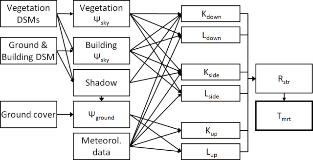
Fig. 12.1 Overview of SOLWEIG
12.2.1.1. Suggested reading
Read the manual and papers listed below to get a full explanation of the model and previous evaluation:
Wallenberg, N., Holmer, B., Lindberg, F., Lönn, J., Maesel, E., and Rayner, D. (2025): A simple step heating approach for wall surface temperature estimation in the SOlar and LongWave Environmental Irradiance Geometry (SOLWEIG) model, EGUsphere [preprint] (link to paper)
Wallenberg, N., Holmer, B., Lindberg, F., and Rayner, D. (2023) An anisotropic scheme for longwave irradiance and its impact on radiant load in urban outdoor settings. International Journal of Biometeorology. (link to paper)
Wallenberg, N., Lindberg, F., Holmer, B., and Thorsson, S. (2020) The Influence of Anisotropic Diffuse Shortwave Radiation on Mean Radiant Temperature in Outdoor Urban Environments.” Urban Climate 31 (2020). (link to paper)
Holmer, B., Lindberg, F., Rayner, D. and Thorsson, S. (2015) How to transform the standing man from a box to a cylinder – a modified methodology to calculate mean radiant temperature in field studies and models, ICUC9 – 9 th International Conference on Urban Climate jointly with 12th Symposium on the Urban Environment, BPH5: Human perception and new indicators. Toulouse, July 2015. (link to paper)
Lindberg, F., Onomura, S. and Grimmond, C.S.B (2016) Influence of ground surface characteristics on the mean radiant temperature in urban areas. International Journal of Biometeorology. 60(9), 1439-1452. (link to paper)
Lindberg, F. and Grimmond, C. (2011) The influence of vegetation and building morphology on shadow patterns and mean radiant temperature in urban areas: model development and evaluation. Theoretical and Applied Climatology 105:3, 311-323. (link to paper)
Lindberg, F., Holmer, B. and Thorsson, S. (2008) SOLWEIG 1.0 – Modelling spatial variations of 3D radiant fluxes and mean radiant temperature in complex urban settings. International Journal of Biometeorology 52, 697–713. (link to paper)
12.2.1.2. Install the model
As SOLWEIG is included in UMEP and UMEP for Processing, follow the Getting Started on how to install QGIS and UMEP. When installed successfully, SOLWEIG is found under UMEP -> Processor -> Outdoor Thermal Comfort -> Mean Radiant Temperature (SOLWEIG). SOLWEIG is also available as a Processing toolbox. Here you can find the most recent version.
12.2.2. Input data
There are two categories of data needed to run SOLWEIG. The first category is the spatial information in the some various raster grids explained below. The other is meteorological data and other settings such as environmental and human exposure parameters.
12.2.2.1. Surface models
One essential prerequisite for performing successful model calculation is that all surface models are of the same extent and pixel resolution.
12.2.2.1.1. Ground and building DSM
As the name suggest this Digital Surface Model (DSM) consist of both ground and building heights in meter above sea level (masl).
12.2.2.1.2. Vegetation DSMs
3D Vegetation is described by two different grids. First a canopy DSM (CDSM) which represents the top of the vegetation and second, a trunk zone DSM (TDSM) that describes the bottom of the vegetation (see schematic figure). Pixel without any 3D vegetation has the value of zero and vegetation pixels are given in meter above ground level (magl). For a detailed description, see Lindberg and Grimmond (2011) [2].
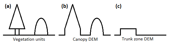
Fig. 12.2 Schematic cross section of the vegetation representation in SOLWEIG. a Conifer tree (left) and bush (right), b the canopy DEM and c trunk zone DEM based on (a). From Lindberg and Grimmond (2011)
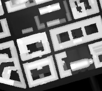
Fig. 12.3 Example of a ground and building DSM
12.2.2.1.3. Digital elevation model
One essential information needed is to know what pixels that are occupied with buildings. In order to locate these pixels, there are two possible ways:
By including a Digital Elevation Model (DEM) (masl) representing only ground elevation which can be used in conjunction with the ground and building DSM to derive building pixels.
By using a land cover grid (see below) where buildings are represented.
If a DEM is used, is has to be the same spatial resolution and extent as all the other grids used.
12.2.2.1.4. Ground cover grid
If the ground cover scheme as presented in Lindberg et al. (2016) [3] should be used, a ground cover grid should be included. The Ground cover grid should be in the UMEP standard format except for the two tree classes (deciduous and conifer). In other words a ground cover grid in SOLWEIG represents what is on the ground surface. A UMEP ground cover grid can be prepared from other data using the Land Cover Reclassifier (UMEP -> Pre-Processor -> Urban Land Cover: Land Cover Reclassifier)
12.2.2.2. Meteorological data
The format and variables used for meteorological data is the same as for other parts of the UMEP-plugin. The time resolution is optional. To prepare such dataset from existing data the Metdata Preprocessor could be used. If no data is available a single point in time can modelled using the SOLWEIG interface. There is also a possibility to download a dataset for any location on Earth using the Download data (ERA5)-plugin. Note that ERA5 data is adjusted to UTC=0. Thus, The UTC offset parameter should also be set to 0 if ERA5 data is used. The variables required for SOLWIEG are:
Air temperature [degC]
Relative humidity [%]
Incoming shortwave radiation [W m-2]
Required are also the components of diffuse and direct-beam shortwave radiation. If these are unavailable, and submodel developed by Reindl et al. (1990) [4] is included in SOLWEIG. Direct radiation perpendicular to the solar beam should be used. If global and diffuse radiation is availalbe, the direct-beam can be calculated using:
direct-beam radiation = (global−diffuse) / sin(sun altitude)
If thermal indicies (PET and UTCI) should be calculated correctly at the POIs (se below), wind speed is required in the forcing data.
12.2.2.3. Environmental parameters
Four main environmental parameters are mandatory; albedo and emissivity of ground and walls. For building walls, these are bulk albedo values with a default of 0.20 (albedo) and 0.90 (emissivity). If the ground cover scheme is not used the bulk ground values are 0.15 (albedo) and 0.95 (emissivity).
If the ground cover scheme is activated (specific tick box found in the plugin-interface), the variables for albedo, emissivity and how surface temperature is parameterised for different surfaces is found in landcoverclasses_v2016a.txt (v2022a). For as detailed description of the ground cover scheme, see Lindberg et al. (2016) [5]. landcoverclasses_v2016a.txt can be found in C:\Users\[you_username]\AppData\Roaming\QGIS\QGIS3\profiles\default\python\plugins\UMEP\SOLWEIG on a Windows PC. As from v2025a a parameter file is introduced, where all setting can be found. This file is located at same location.
It should be noted that it is only grass and impervious surfaces that has been parameterisised and evaluated. Other surfaces such as bare soil and water are only first order approximations at this point.
There is a possibility to include upto 20 ground cover classes in landcoverclasses_v2016a.txt. Ground cover codes upto 20 can be added. The table below specify the information needed in landcoverclasses_v2016a.txt:
Alb Emis Ts_deg Tstart TmaxLST
Column |
Description |
|---|---|
Name |
Any name to identify type of ground cover |
Code |
The values that should be used in ground cover raster to identify type |
Alb |
Albedo |
Emis |
Emmissivity |
Ts_deg |
Increace of Ts per degree max sun altitude during clear weather (k in linerar eq.) |
Tstart |
Start temperature at sunrise (m in linerar eq.) |
TmaxLST |
Time during the day when maximum Ts is reached |
As from v2026a, a new ground cover scheme will be introduced using a Force/Restore method to derive ground surface temperature. This method is more physically based than the previous method and will also include estimation to Ts during night which was not the case for the earlier scheme. This method use more common parameters such as heat capacity and conduction to derive Tsurface. A manuscript is under production.
12.2.2.4. Human exposure parameters
There are three human exposure parameters available:
Absorption of shortwave radiation (default value=0.70)
Absorption of longwave radiation (default value=0.95)
Posture (default value=Standing)
12.2.2.5. Optional settings
The original model as described in Lindberg et al. (2008) [6] used an adjustment of sky emissivity (Jonsson et al. (2006) [7] calculated using the method presented in Prata (1996) [8]. This is now removed but can be added as an option.
As from version 2015a it is possible to consider the human as a cyliner instead of a box. See Holmer et al. (2015) [9] for more details.
12.2.3. Output data
There are two forms of output available, calculated grids of various parameters and full model outputs from certain point of interests (POIs) within the model domain.
12.2.3.1. Surface grids
There are six different grids that can be saved from each model iteration:
Mean radiation temperature
Incoming shortwave radiation
Outgoing shortwave radiation
Incoming longwave radiation
Outgoing longwave radiation
Shadow patterns
A post-processing plugin (SOLWEIG Analyzer) for the output grids are planned to be included in future versions of UMEP.
12.2.3.2. POI.txt
By ticking in the option to include POIs (Point of Interest), a vector point layer can be added and full model output are written out to text files for the specific POI. Multiple POIs can be used by including many points in the vector file. In the table below is the output variables specifiedː
Column |
Name |
Description |
|---|---|---|
1 |
iy |
Year [YYYY] |
2 |
id |
Day of year [DOY] |
3 |
it |
Hour [H] |
4 |
imin |
Minute [M] |
5 |
dectime |
Decimal time [-] |
6 |
altitude |
altitude of the Sun [°] |
7 |
azimuth |
azimuth of the Sun [°] |
8 |
kdir |
direct beam solar radiation (from meteorological data) [W m-2] |
9 |
kdiff |
diffuse component of radiation (from meteorological data) [W m-2] |
10 |
kglobal |
global radiation (from meteorological data) [W m-2] |
11 |
kdown |
Incoming shortwave radiation [W m-2] |
12 |
kup |
Outgoing shortwave radiation [W m-2] |
13 |
keast |
Incoming shortwave radiation [W m-2] |
14 |
ksouth |
Outgoing shortwave radiation [W m-2] |
15 |
kwest |
Incoming shortwave radiation [W m-2] |
16 |
knorth |
Outgoing shortwave radiation [W m-2] |
17 |
ldown |
Incoming longwave radiation [W m-2] |
18 |
lup |
Outgoing longwave radiation [W m-2] |
19 |
least |
Incoming longwave radiation [W m-2] |
20 |
lsouth |
Outgoing longwave radiation [W m-2] |
21 |
lwest |
Incoming longwave radiation [W m-2] |
22 |
lnorth |
Outgoing longwave radiation [W m-2] |
23 |
Ta |
air temperature from meteorological data [°C] |
24 |
Tg |
calculated surface temperature [°C] |
25 |
RH |
relative humidity from meteorological data [percent] |
26 |
Esky |
sky emissivity |
27 |
Tmrt |
mean radiant temperature [°C] |
28 |
I0 |
theoretical value of maximum incoming solar radiation [W m-2] |
29 |
CI |
clearness index |
30 |
Shadow |
Shadow value |
31 |
SVF_b |
Sky View Factor from ground and buildings |
32 |
SVF_b+v |
Sky View Factor from ground, buildings and vegetation |
33 |
KsideI |
Direct shortwave radiation from side if cylinder option is used |
34 |
PET |
Phyciological Equivalent Temperature |
35 |
UTCI |
Universal Thermal Comfort Index |
12.2.4. GPU acceleration
SOLWEIG supports GPU acceleration to speed up calculations. Using a graphics card to speed up SOLWEIG solar radiation calculations works best under specific conditions. For smaller datasets, the extra time required to transfer your data over to the GPU can be larger than the actual calculation time. This means you will mostly see a clear benefit when you process geographic areas that span more than a few square kilometers, or when you use high-resolution input data. Small datasets might show no performance gain at all. Your choice of hardware also plays a major role, since newer and more powerful graphics cards provide much better speedup than older models.
12.2.4.1. Supported Hardware
The system supports hardware acceleration across a variety of graphics processing units. This includes dedicated NVIDIA graphics cards as well as Intel graphics systems. If you’re using an AMD GPU, you must setup AMD ROCM on your machine for your GPU to be utilized. Sweeping performance gains are highly dependent on your specific model, where modern and advanced GPUs deliver the highest efficiency.
12.2.4.2. Requirements
Using the GPU acceleration functionality requires a compatible graphics card and a functional PyTorch installation. Additionally, your graphics drivers must be up to date to ensure the system communicates correctly with your hardware and runs calculations efficiently. To install, use pip install torch OR directly from the OSgeo4W setup.
12.2.4.3. Memory Management
The software takes care of all memory management behind the scenes. As soon as the GPU-accelerated solar radiation calculations are complete, the system automatically wipes the graphics memory. This ensures your hardware is immediately ready for other applications, and it requires no manual effort from you.
12.2.4.4. Troubleshooting
If your processing task stops because of an out-of-memory error, you can fix this by shrinking your input dataset or disabling the graphics acceleration entirely. Graphics cards generally have less memory capacity than standard system RAM, meaning massive datasets can easily exceed the hardware limits. If you have to process a very large region, dividing the area into several smaller tiles is a highly effective solution.
Also, some times on the QGIS version the VRAM is not cleared properly after use, so try to restart QGIS to free it.
If the GPU selection is visible but causes an error when you try to run it, you should double-check your PyTorch installation. If you have just updated your operating system or installed a new graphics driver, a fresh reinstallation of PyTorch usually fixes the problem.
If the simulation feels slower with the GPU turned on compared to the CPU, this is typical behavior for small datasets where the setup overhead is larger than the computation time. We recommend turning the GPU off for minor tasks and turning it on only for large-scale simulations.
To keep your system running smoothly, make sure your graphics drivers stay updated via your manufacturer’s website.
12.2.4.5. Backward Compatibility
The addition of GPU support does not affect older workflows because the system is designed with full backward compatibility. You are never forced to use the graphics card features. If you do not have PyTorch installed, or if your computer lacks the right hardware, the algorithms will seamlessly fall back to CPU computation. All of your older projects and saved scripts will run perfectly without requiring any modifications.
12.2.5. How to run the model
The following section provides information on how to run the model and what consideration that should be taken into account in order for the model to perform at its best.
12.2.5.1. Run the model for example data
Before running the model for your own data it is good to make certain that you can run the test data and get the same results as in the example files provided. Test/example files are given for Göteborg, Sweden or London, UK. Here, you will use the Göteborg data.
Download and extract the Gothenburg test dataset to your computer.
Add the raster layers (DSM, CDSM and land cover) from the Goteborg folder into a new QGIS session. The coordinate system of the grids is Sweref99 1200 (EPSG:3007).
In order to run SOLWEIG, some additional datasets must be created based on the raster grids you just added. Open the SkyViewFactor Calculator from the UMEP Pre-processor and calculate SVFs using both your DSM and CDSM. Leave all settings as default. This calculation produces a file called ‘svf.zip’ which is used later in the calculations.
Open the Wall height and aspect plugin from the UMEP Pre-processor and calculate both wall height and aspect using the DSM and your input raster. Make sure to add the result to your project.
Now you are ready to generate your first Tmrt map. Open SOLWEIG and use the settings as shown below but replacing the paths to fit your computer environment. When you are finished, press Run.
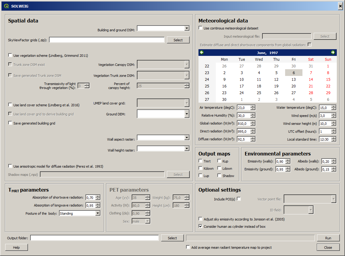
Fig. 12.4 Dialog for the SOLWEIG model (version 2022a found in the menu-based UMEP plugin).
12.2.6. Tips and Tricks
All grids must have the same extent and pixel resolution.
The coordinate system of all the grids must be the same and translatable to lat, lon coordinates.
Meteorological file must have the default UMEP format.
Wall height and aspect grids as well as SVFs can be calculated from Pre-processor in UMEP.
The model is very sensitive to the timing global radiation, i.e.. that the peak of solar radiation occurs at local noon. If using a meteorological file included a longer dataset, this could be checked by comparing the global solar radiation and the theoretical maximum of solar radiation (I0) from a solar exposed point of interest.
Land cover grid should be in UMEP format.
A boolean building grid (building = 0, ground = 1) is used in the model. This grid is created either from the land cover grid or the ground DEM in conjunction with the building and ground DSM.
If using the land cover grid to derive the building grid, it is important that it coincides with the ground and building DSM. Otherwise strange results will be produced.
SOLWEIG focus on pedestrian radiation fluxes and it is not recommended to consider fluxes on building roofs.
12.2.7. Acknowledgements
People who have contributed to the development of SOLWEIG (plus co-authors of papers):
Current contributors:
Nils Wallenberg (University of Gothenburg, Sweden)
C.S.B. Grimmond (University of Reading; previously Indiana University, King’s College London, UK),
Fredrik Lindberg (University of Gothenburg, Sweden)
Björn Holmer (University of Gothenburg, Sweden)
Jessika Lönn (University of Gothenburg, Sweden)
Past Contributors:
Shiho Onomura (University of Gothenburg)
Sofia Thorsson (University of Gothenburg)
Ingegärd Eliasson (University of Gothenburg)
Janina Konarska (University of Gothenburg)
David Rayner (University of Gothenburg)
Funding to support development:
FORMAS, National Science Foundation (USA, BCS-0095284, ATM-0710631), EU Framework 7 BRIDGE (211345); EU emBRACE; UK Met Office; NERC ClearfLO, NERC TRUC.
12.2.8. Abbreviations
DEM |
Digital Elevation Model |
|---|---|
DSM |
Digital surface model |
DTM |
Digital Terrain Model |
L↓ |
Incoming longwave radiation |
LAI |
Leaf area index |
SOLWEIG |
The solar and longwave environmental irradiance geometry model |
SVF |
Sky view factor |
UMEP |
|
GUI |
Graphical User Interface |
POI |
Point of Interest |
12.2.9. Development
SOLWEIG is an an open source model that we are keen to get others inputs and contributions. There are two main ways to contribute:
Submit comments or issues to the issue tracker
Participate in Coding or adding new features DevelopmentGuidelines.
12.2.10. Version History
Version |
Changes from previous version |
|---|---|
v2026a (Under development) |
Introducing a surface temperature scheme appying a force/restore method. |
v2025a |
Introducing a new wall surface temperature scheme according to Wallenberg et al. (2025) [12]. Also, compatible with QGIS 4. |
v2022a |
Introducing anisotropic longwave radiation according to Wallenberg et al. (2023) [11]. |
v2021a |
Bug fixes and small improvements. See https://github.com/UMEP-dev/UMEP for more details. |
v2019a |
Possibilities to make use of an anisotropic diffuse shortwave scheme (Wallenberg et al. 2020) [10] is added. |
v2018a |
Minor bug fixing in ground view factor calculation. Introduction to PET and UTCI calculations for POIs. Available only for QGIS3. |
v2016a |
First version released within UMEP. Python version of model is now released as open source. |
v2015a |
|
v2014a |
|
2013a |
A new GUI is introduced as well as options to load gridded vegetation DSMs. |
2.3 |
A new scheme for reflection concerning the shortwave fluxes is included taking into account sunlit and shaded walls |
2.2 |
Some major (and minor) bugs have been fixed such as: * - - A major bug regarding the scale of trees and bushes is resolved |
2.0 |
A new vegetation scheme is now included (Lindberg and Grimmond 2011). The interface also has a wizard for generating vegetation data to be included in the calculations. The new vegetation scheme is again slowing down the calculation but the computation time is still acceptable. |
1.1 |
Longwave and shortwave radiation fluxes from the four cardinal points is now separated based on anisotropical Sky View Factor (SVF) images. Ground View Factors is introduced which is a parameter that is estimated based on what an instrument measuring Lup actually is seeing based on its height above ground and shadow patterns. In order to make accurate estimations of GVF, locations of building walls need to be known. Walls can be found automatically be the SOLWEIG-model. However, if the User wants to have more control over what are buildings and not, the User should use the marking tool included in the ‘Create/Edit Vegetation DEM’. A very simple approach taken from Offerle et al. (2003) is used to estimate nocturnal Ldown. Therefore Tmrt could also be estimated during night in version 1.1. |
1.0 |
First version as from Lindberg et al. (2008) |