Thermal Comfort - Introduction to SOLWEIG
Note
Click here to find the same tutorial as below but for data from New York City, US.
Introduction
In this tutorial you will use a model SOlar and LongWave Environmental Irradiance Geometry model (SOLWEIG) to estimate the mean radiant temperature (Tmrt).
SOLWEIG is a model that simulates spatial variations of 3D radiation fluxes and the Tmrt in complex urban settings. It is also able to model spatial variations of shadow patterns. Tmrt is one of the key meteorological variables governing human energy balance and the thermal comfort of people. It is derived from summing all the radiative (shortwave and longwave) fluxes (both direct and reflected) to which the human body is exposed. In SOLWEIG, Tmrt is derived by modelling shortwave and longwave radiation fluxes in six directions (upward, downward and from the four cardinal points) and angular factors.
The model requires meteorological forcing data (global shortwave radiation (Kdown), air temperature (Ta), relative humidity (RH)), urban geometry (DSMs), and geographic information (latitude, longitude and elevation). To determine Tmrt, continuous maps of sky view factors are required. Both vegetation and ground cover information can be added to increase the accuracy of the model output. Below, a schematic flowchart of SOLWEIG in shown. The full manual provides more detail.
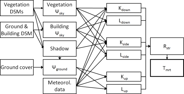
Fig. 99 Overview of SOLWEIG
Objectives
To introduce SOLWEIG and how to run the model within UMEP (Urban Multi-scale Environmental Predictor).
Help with Abbreviations can be found here.
Steps
Different kinds of input data, that are needed to run the model, will be generated.
How to run the model
How to examine the model output
Add additional information (vegetation and ground cover) to improve the model outcome and to examine the effect of climate sensitive design
Initial Practical steps
UMEP is a python plugin used in conjunction with QGIS. To install the software and the UMEP plugin see the getting started section in the UMEP manual.
As UMEP is under constant development, some documentation may be missing and/or there may be instability. Please report any issues or suggestions to our repository.
Data for this exercise
The UMEP tutorial datasets can be downloaded from our here repository here.
Download, extract and add the raster layers (DSM, CDSM, DEM and land cover) from the Goteborg folder into a new QGIS session (see below).
Create a new project
Examine the geodata by adding the layers (DSM_KRbig, CDSM_KRbig, DEM_KRbig and landcover) to your project (*Layer > Add Layer > Add Raster Layer).
Coordinate system of the grids is Sweref99 1200 (EPSG:3007). If you look at the lower right hand side you can see the CRS used in the current QGIS project.
Have a look at A First QGIS and UMEP activity on how you can visulaise DSM and CDSM at the same time.
Examine the different datasets before you move on.
To add a legend to the land cover raster you can load landcoverstyle.qml found in the test dataset. Right click on the land cover (Properties -> Style (lower left) -> Load Style).
SOLWEIG Model Inputs
Details of the model inputs and outputs are provided in the SOLWEIG manual. As this tutorial is concerned with a simple application only the most critical parameters are used. Many other parameters can be modified to more appropriate values, if applicable. The table below provides an overview of the parameters that can be modified in the Simple application of SOLWEIG.
Data use and type abbreviations: R: required, O: Optional, N : not needed, S: Spatial, M: Meteorological,
Data |
Definition |
Use |
Type |
Description |
Ground and building digital surface model (DSM) |
High resolution surface model of ground and building heights |
R |
S |
Given in metres above sea level (m asl) |
Digital elevation model (DEM) |
High resolution surface model of the ground |
R* |
S |
R* if land cover is absent to identify buildings. Given in m asl. Must be same resolution as the DSM. |
Digital canopy surface model (CDSM) |
High resolution surface model of 3D vegetation |
O |
S |
Given in metres above ground level (m agl). Must be same resolution as the DSM. |
Digital trunk zone surface model (TDSM) |
High resolution surface model of trunk zone heights (underneath tree canopy) |
O |
S |
Given in m agl. Must be same resolution as the DSM. |
Land (ground) cover information (LC) |
High resolution surface model of ground cover |
O |
S |
Must be same resolution as the DSM. Five different ground covers are currently available (building, paved, grass, bare soil and water) |
UMEP formatted meteorological data |
Meteorological data from one nearby observation station, preferably at 1-2 m above ground. |
R |
M |
Any time resolution can be given. |
Latitude (°) |
Solar related calculations |
R |
O |
Obtained from the ground and building DSM coordinate system |
Longitude (°) |
Solar related calculations |
R |
O |
Obtained from the ground and building DSM coordinate system |
Time zone |
R |
O |
Influences solar related calculations. Set in the interface of the model. |
|
Human exposure parameters |
Absorption of radiation and posture |
R |
O |
Set in the interface of the model. |
Environmental parameters |
e.g. albedos and emissivites of surrounding urban fabrics |
R |
O |
Set in the interface of the model. |
Meterological input data should be in UMEP format. You can use the Meterological Preprocessor to prepare your input data. It is also possible use the plugin for a single point in time.
Required meteorological data to calculate Tmrt is:
Air temperature (°C)
Relative humidity (%)
Incoming shortwave radiation (W m2)
The model performance will increase if diffuse and direct beam solar radiation is available but the mdoel can also calculate these variables.
If Point Of Interest (POIs) is used, wind speed (m/s) is also required (see below).
How to Run SOLWEIG from the UMEP-plugin
Open SOLWEIG from UMEP -> Processor -> Outdoor Thermal Comfort -> Mean radiant temperature (SOLWEIG).
You will make use of a test dataset from observations for Gothenburg, Sweden.
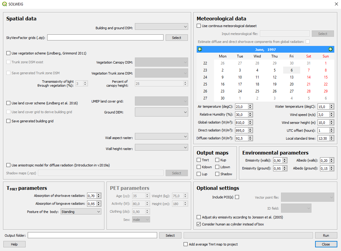
Fig. 100 Dialog for the SOLWEIG model (click on figure for larger image)
To be able to run the model, some additional spatial datasets needs to be created.
Close the SOLWEIG plugin and open UMEP from the processing toolbox then Pre-Processor -> Urban geometry: Sky View Factor.
To run SOLWEIG various sky view factor (SVF) maps for both vegetation and buildings must be created (see Lindberg and Grimmond (2011) for details).
You can create all SVFs needed (vegetation and buildings) at the same time. Use the settings as shown below. Use an appropriate output folder for your computer.
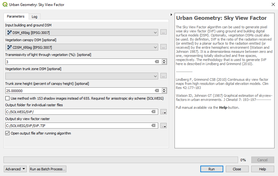
Fig. 101 Settings for the SkyViewFactorCalculator.
When the calculation is done, a map will appear in the map canvas. This is the ‘total’ SVF i.e., including both buildings and vegetation. Examine the dataset.
Where are the highest and lowest values found?
If you look in your output folder you will find a zip-file containing all the necessary SVF maps needed to run the SOLWEIG-model.
Another preprocessing plugin is needed to create the building wall heights and aspect. Open UMEP from the processing toolbox again and then Pre-Processor -> Urban geometry: Wall height and aspect and use the settings as shown below. QGIS scales loaded rasters by a cumulative count out approach (98%). As the height and aspect layers are filled with zeros where no wall are present it might appear as if there is no walls identified. Rescale your results to see the walls identified (Layer Properties > Symbology).
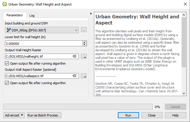
Fig. 102 Settings for the Wall height and aspect plugin.
Re-open the SOLWEIG plugin and use the settings shown below. You will use the GUI to set one point in time (i.e. a summer hour in Gothenburg, Sweden) hence, no input meteorological file is needed for now. No information on vegetation or ground cover is added for this first try. Click Run.
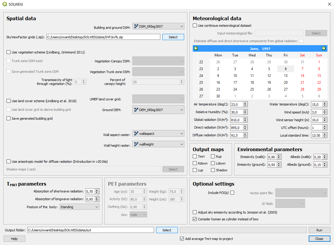
Fig. 103 The settings for your first SOLWEIG run (click on figure for larger image).
Examine the output (Average Tmrt (°C). What is the main driver to the spatial variations in Tmrt?
Add 3D vegetation information by ticking Use vegetation scheme (Lindberg, Grimmond 2011) and add CDSM_Krbig as the Vegetation Canopy DSM. As no TDSM exists we estimate it by using 25% of the canopy height. Leave the tranmissivity as 3%. Tick Save generated Trunk Zone DSM (a tif file, TDSM.tif, will be generated in the specified output folder and used in a later section: Climate sensitive planning). Also tick Save generated building grid as this will be needed later in this tutorial. Leave the other settings as before (Step 4) except for changing your output directory, otherwise results from your first run will be overwritten. Run the model again and compare the result with your first run.
Add your last spatial dataset, the land cover grid by ticking Use land cover scheme (Lindberg et al. 2016). Run and compare the result again with the previous runs.
Using meteorolgical data and POIs
SOLWEIG is also able to run a continuous dataset of meteorological data. You will make use of a single summer day as well as a winter day for Gothenburg, Sweden. The GUI is also able to derive full model output (all calculated variables) from certain points of interest (POIs).
First you need to create a point vector layer to store the POIs. Go to Layer > Create Layer > New Shape file. Choose Point as Type and add a new text field called name. Name the new layer POI_Kr.shp. Specify the coordinate system as SWEREF99 12 00 (EPSG: 3007).
Now you should add two points within the study area. To add points to the layer it has to be editable and Add Feature should be activated.

Fig. 104 Settings to add points
Two points should be added and the attributes should be id=1 and name=courtyard for the right point and id=2 and name=park for the left point. See figure below for the locations of the two points.
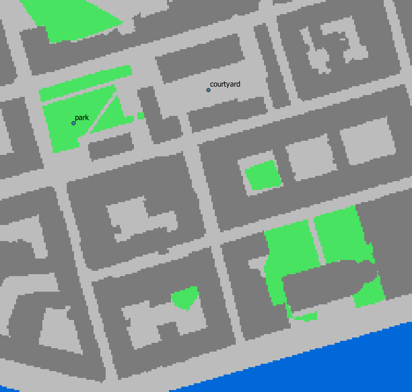
Fig. 105 Location of the two POIs
When you are finished, save layer edits (box in-between the two marked boxes in Figure 6). Close the editing by pressing Toggle editing (the pencil).
Now open the SOLWEIG plugin. Use both the vegetation and land cover schemes as before. This time, tick in Include POI(s), select your point layer and use the ID attribute as ID field.
Tick in Use continuous meteorological dataset and choose gbg19970606_2015a.txt as Input meteorological file. Also, tick in to save Tmrt (in the Output maps section of the dialogue box). Run the model again.
Examine your output with SOLWEIG Analyzer
To perform a first set of analysis of your result you can make use of the SOLWEIG Analyzer plug-in.
Open the Analyzer located in UMEP -> Post-Processor -> Outdoor Thermal Comfort -> SOLWEIG Analyzer. Here you can analyze both data from your POIs as well as perform statistical analysis based on saved output maps. Start by locating your output folder in the top section (Load Model Result).
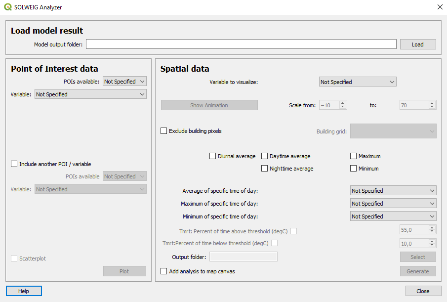
Fig. 106 Dialog for the SOLWEIG Analyzer plug-in
Firstly you will compare differences in Tmrt for the two locations (courtyard and park). This can done using the left frame (Point of Interest data). Specify courtyard (1) as the POI and Mean Radiant Temperature as the variable in the two top scroll down lists. Then tick in Include another POI/variable and chose park (2) and Mean Radiant Temperature below. Click Plot. What explains the differences?
Now lets move on to analyse the output maps generated from our last model run. In the right frame, specify Mean Radiant Temperature as Variable to visualize. Start by clicking Show Animation. Now the output maps of Tmrt generated before are displayed in a sequence.
The next step is to generate some statistical maps from the last model run. Specify Mean Radiant Temperature as Variable to visualize and tick Exclude building pixels. Choose the building grid that you saved earlier in this tutorial. If it is not in the drop-down list you need to add this layer (buildings) to your project. Tick in Tmrt Percent of time above threshold (degC) and specify 55.0 as threshold. Specify an output folder and also tick Add analysis to map canvas before you generate the result. The resulting map show the time that a pixel has been above 55 degC based on the whole analysis time i.e. 24 hours. This type of map can be used to identify areas prone to heat stress, for example.
Climate sensitive planning
Vegetation is one effective measure to reduce areas prone to heat related health issues. In this section you make use of the Tree Generator plugin to see the effect of adding more vegetation into our study area. The municipality in Gothenburg have identified a “hot spot” south of the German church and they want to see the effect of planting three new trees in that area.
The Tree Generator
The Tree Generator plugin makes use of a point vector file including the necessary attributes to generate/add/remove vegetation suitable for either mean radiant temperature modelling with SOLWEIG or urban energy balance modelling with SUEWS.
Create a point vector shape file named (TreesKR.shp), as described in the previous section, adding five attributes (id, ttype, trunk, totheight, diameter). The attributes should all be decimal (float) numbers (see table below). The location of the three new trees are shown in figure below. The values for all three vegetation units should be ttype=2, trunk=4, totheight=15, diameter=10.
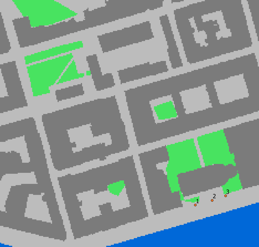
Fig. 107 Location of the three new vegetation units.
Add your created trunk zone dsm (tdsm.tif) that was created previously (located in your output directory).
Open the TreeGenerator (UMEP > PreProcessor > Spatial Data > TreeGenerator) and use the settings as shown in figure below.
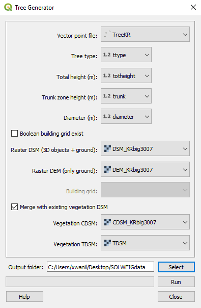
Fig. 108 The settings for the Tree Generator
As the vegetation DSMs have been changed, the SVFs have to be recalculated. This time use the two generated vegetation DSMs.
Re-run SOLWEIG using the same settings as before but now use the new vegetation surface models as well as the new SVFs generated in the previous step.
Generate a new, updated threshold map based on the new results and compare the differences.
The table below show the input variables needed for each tree point.
Attribute name |
Name |
Description |
|---|---|---|
ttype |
Tree type |
Two shapes are available:
|
trunk |
Trunk zone height (m agl) |
Height of the trunk zone. |
totheight |
Total tree height (m agl) |
Maximum height of the vegetation unit |
diameter |
Canopy diameter (m) |
Circular diameter of the vegetation unit |
Tutorial finished.