Writing Python scripts for GIS applications can make your GIS life much easier. Especially when you want to automate various GIS processes or analyses. In this tutorial you will take your first steps in using UMEP tools in a Python script to create an aggregated shadow map generated over mutiple days.
This tutorial consists of two parts:
Create a loop script in the Python editor in QIGS which generates mutiple shadows on a Digital Surface Model (DSM).
Learn how to write a standalone script outside of QGIS in Windows. Here we use of Jupyter Notebook as the integrated development environment (IDE).
The UMEP tutorial datasets can be downloaded from our here repository here.
Download, extract and add the two raster layers (DSM, CDSM) from the Goteborg folder into a new QGIS session.
It is also essential that the raster datasets are set to the correct coordinate system before running the Shadow Generator which is SWEREF99 1200 (EPSG:3007).
First make sure that you have installed UMEP for processing from the Plugins>Manage and Install Plugins. Then open the QGIS Python Console from Plugins>Python Console. From here you can access the Editor by clicking on the symbol with a sheet of paper and a pen. Here we can write Python code and execute Python command as a script.
After loading the raster datasets into QGIS and downloading UMEP for processing it is
necessary to run the tool Shadow generator from UMEP for Processing which can be found in
the Processing Toolbox under UMEP>Processor>Solar Radiation: Shadow Generator (same tool as Daily Shadow Patterns in menu-based UMEP). You will first execute the Shadow Generator to obtain the input information for the Shadow generator.
The settings in the Shadow Generator are set accordingly:
Input DSM as DSM_KRbig
Vegetation Canopy DSM as CDSM_KRbig
UTC = 1
Leaving Vegetation Transmissivity, Time, Date and the rest as it is.
When the algorithm is done, go to the Log-tab and copy the lines underneath the input parameters:
These inputs will be used later to develop the script that we need. Note that your paths to INPUT_DSM and INPUT_CDSM are different. The Shadow Generator only allows you to choose one date, UTC and Light Transmissivity percentage but with the Python Script it will be possible to run the tool for several dates and different settings.
Paste everything in an empty script in the Editor and save it as MyFirstPythopnScript.py. You can execute it by clicking the green arrow above the Editor but nothing exciting will happen since the script really does not do anything yet. We first should create a variable of the pasted text by adding parin = * before the first curly bracket. Then also add *print(parin) at the end of your script. Remember that Python is intendent sensitive to the print statement must start at the beginning of a row. Execute again and the parin variable will print out in the QGIS Python console. Still not very exciting. We do not really need to print the parin variable so we can comment this line out by adding a # in the beginning of that line. To execute the Shadow casting algorithm you need to add processing.run(“umep:Solar Radiation: Shadow Generator”, parin) at the end of your script.
You can change the settings for the Shadow casting algorithm as you wish now. For example, change the OUTPUT_DIR to “C:/temp/shadowmaps/”. You also need to create such folder on your system. If you don’t have right to create a folder such as C:/temp/shadowmaps/ you can create the shadowmaps folder on your desktop. If you now execute your script you will see a number of tif-files in your shadowmaps folder. Before you move on, make sure that your shadowmaps folder is empty.
The next step is to figure out how to write a date loop in a way that the tool can be run for several dates at the same time. The date variable in the loop has to be written in a way that matches the date from the Shadow Generator input parameters.
The DATEINI parameter is a QDate variable which is used in QGIS. To create such variable, you can make use of a method enbedded in the QDate object. Write the following at the beginning of your code:
datetorun=QDate.fromString("4-5-2015","d-M-yyyy")
Now change your DATEINI variable to datetorun as shown below and execute your script. Now your should see a number of geotifs in your shadowmaps-folder with the date 20150405 specified. Again, delete those files.
Now, temporally comment out the line with your processing.run statement (#), as we need to try to adjust the time variable. We will make use of the datetime module in Python. In order to access datetime, you need to import the module by adding import datetime at the top of your script.
Also add three more variables defining the start date of your analysis:
startyear=2022startmonth=4startday=1
Now, you will create a loop so that the script will execute the shadow casting algorithm for a number of days in sequence. Important when working with loops (and statements) in Python is to indent the code within a loop. We will try to make a for-loop starting after the startday variable:
Execute (a sequence of 10 dates starting from April 1, 2022 should be displayed in the Python console).
Moving on, now we need to include the shadow casting algorithm within the loop we have just created. This is done by indenting the parin variable, the processing.run statement and the datetorun variable. Do not forget to uncomment your processing.run statement at this point. You also need to change the datetorun variable to include the new date variable:
datetorun=QDate.fromString(date,"d-M-yyyy")
We also want to add capabilities to adjust for off-leaf, on-leaf periods of the year. This is done by adding an if-statement changing the TRANS_VEG variable in parin. Within the for-loop, add the following (and do not forget about indentation):
Also add the transVeg variable as input for TRANS_VEG in the parin dictionary.
Next step is to add all the shadow images into one aggregated raster. In the for-loop, after the processing.run statement, add the following code:
no_of_files=os.listdir('c:/temp/shadowmaps/')forjinrange(0,no_of_files.__len__()):tempgdal=gdal.Open('c:/temp/shadowmaps/'+no_of_files[j])Tempraster=tempgdal.ReadAsArray().astype(float)fillraster=fillraster+Temprastertempgdal=Noneos.remove('c:/temp/shadowmaps/'+no_of_files[j])index=index+1#A counter that specifies total number of shadows in a year (30 minute resolution)
As you can see you can also add comments in the code, to specify what is happening in the code. The lines above should be within the main for-loop, a so-called nested loop (a loop within a loop) so remember to use the correct indentation. Some new variables is found in this nested for-loop. These need to be defined before the main loop, at the top of the code. One of these new variables is an empty raster (fillraster) that will be used to aggregate all the shadow images generated.
When the nested loop is done, fillraster should be normalised by the number of iterations:
fillraster=fillraster/index
Your script should now look like this:
importdatetimestartyear=2022startmonth=3startday=15index=0baseraster=gdal.Open('C:/Users/xlinfr/Documents/PythonScripts/SOLWEIG/SOLWEIGdata/DSM_KRbig.tif')fillraster=baseraster.ReadAsArray().astype(float)fillraster=fillraster*0.0foriinrange(0,10):date=datetime.date(startyear,startmonth,startday)+datetime.timedelta(days=i)date=date.strftime("%d-%m-%Y")print(date)datetorun=QDate.fromString(date,"d-M-yyyy")if(datetorun>QDate(startyear,4,15))&(datetorun<QDate(startyear,10,1)):transVeg=3else:transVeg=49parin={'DATEINI':datetorun,'DST':False,'INPUT_ASPECT':None,'INPUT_CDSM':'C:/Users/xlinfr/Documents/PythonScripts/SOLWEIG/SOLWEIGdata/CDSM_KRbig.asc','INPUT_DSM':'C:/Users/xlinfr/Documents/PythonScripts/SOLWEIG/SOLWEIGdata/DSM_KRbig.tif','INPUT_HEIGHT':None,'INPUT_TDSM':None,'INPUT_THEIGHT':25,'ITERTIME':30,'ONE_SHADOW':False,'OUTPUT_DIR':'c:/temp/shadowmaps/','TIMEINI':QTime(16,32,58),'TRANS_VEG':transVeg,'UTC':1}processing.run("umep:Solar Radiation: Shadow Generator",parin)no_of_files=os.listdir('c:/temp/shadowmaps/')forjinrange(0,no_of_files.__len__()):tempgdal=gdal.Open('c:/temp/shadowmaps/'+no_of_files[j])tempraster=tempgdal.ReadAsArray().astype(float)fillraster=fillraster+temprastertempgdal=Noneos.remove('c:/temp/shadowmaps/'+no_of_files[j])index=index+1#A counter that specifies total numer of shadows in a year (30 min resolution)fillraster=fillraster/index
The last thing we need to do is to save fillraster as a geotiff. Here, we will make use of a function that we will create. This makes it possible to later reuse the same code when needed. A function in Python is recognised by starting with def followed by indented lines of code included in the function. At the top of your script, after your imports, add the following:
defsaveraster(gdal_data,filename,raster):rows=gdal_data.RasterYSizecols=gdal_data.RasterXSizeoutDs=gdal.GetDriverByName("GTiff").Create(filename,cols,rows,int(1),GDT_Float32)outBand=outDs.GetRasterBand(1)# write the dataoutBand.WriteArray(raster,0,0)# flush data to disk, set the NoData value and calculate statsoutBand.FlushCache()outBand.SetNoDataValue(-9999)# georeference the image and set the projectionoutDs.SetGeoTransform(gdal_data.GetGeoTransform())outDs.SetProjection(gdal_data.GetProjection())
And at the end of your code, lets call this function:
Last thing we should add is a variable that decides how many days that we want to examine. Before your for-loop, put in:
noofdays=10
Then change your first for statement to:
foriinrange(0,noofdays):
Here is your final script:
importdatetimefromosgeoimportgdalimportnumpyasnpfromosgeo.gdalconstimport*defsaveraster(gdal_data,filename,raster):rows=gdal_data.RasterYSizecols=gdal_data.RasterXSizeoutDs=gdal.GetDriverByName("GTiff").Create(filename,cols,rows,int(1),GDT_Float32)outBand=outDs.GetRasterBand(1)# write the dataoutBand.WriteArray(raster,0,0)# flush data to disk, set the NoData value and calculate statsoutBand.FlushCache()outBand.SetNoDataValue(-9999)# georeference the image and set the projectionoutDs.SetGeoTransform(gdal_data.GetGeoTransform())outDs.SetProjection(gdal_data.GetProjection())startyear=2022startmonth=3startday=15index=0noofdays=10baseraster=gdal.Open('C:/Users/xlinfr/Documents/PythonScripts/SOLWEIG/SOLWEIGdata/DSM_KRbig.tif')fillraster=baseraster.ReadAsArray().astype(float)fillraster=fillraster*0.0foriinrange(0,noofdays):date=datetime.date(startyear,startmonth,startday)+datetime.timedelta(days=i)date=date.strftime("%d-%m-%Y")print(date)datetorun=QDate.fromString(date,"d-M-yyyy")if(datetorun>QDate(startyear,4,15))&(datetorun<QDate(startyear,10,1)):transVeg=3else:transVeg=49parin={'DATEINI':datetorun,'DST':False,'INPUT_ASPECT':None,'INPUT_CDSM':'C:/Users/xlinfr/Documents/PythonScripts/SOLWEIG/SOLWEIGdata/CDSM_KRbig.asc','INPUT_DSM':'C:/Users/xlinfr/Documents/PythonScripts/SOLWEIG/SOLWEIGdata/DSM_KRbig.tif','INPUT_HEIGHT':None,'INPUT_TDSM':None,'INPUT_THEIGHT':25,'ITERTIME':30,'ONE_SHADOW':False,'OUTPUT_DIR':'c:/temp/shadowmaps/','TIMEINI':QTime(16,32,58),'TRANS_VEG':transVeg,'UTC':1}processing.run("umep:Solar Radiation: Shadow Generator",parin)no_of_files=os.listdir('c:/temp/shadowmaps/')forjinrange(0,no_of_files.__len__()):tempgdal=gdal.Open('c:/temp/shadowmaps/'+no_of_files[j])tempraster=tempgdal.ReadAsArray().astype(float)fillraster=fillraster+temprastertempgdal=Noneos.remove('c:/temp/shadowmaps/'+no_of_files[j])index=index+1#A counter that specifies total numer of shadows in a year (30 minute resolution)fillraster=fillraster/indexsaveraster(baseraster,'c:/temp/Shadow_Aggregated.tif',fillraster)
Now you can execute and wait for the final result. When the script is done, load Shadow_Aggragated.tif in QGIS and examine the result.
As you might have noticed, QGIS freeze when running a script that requires some time to finish. Therefore, it might be useful to run QGIS-related scripts “outside” of QGIS.
In this section we will explain a method to execute the script we just created in a Jupyter Notebook. There are also other so called IDEs for writing and running Python code, e.g. PyCharm, VSCode, Spyder/Anaconda etc. Jupyter Notebook can be accessed from a webbrowser which can be convenient.
First we need to install Jupyter and configure our environment so that all OSGeo components are recognised by the notebook.
This method requires that you have installed QGIS according to the recommendation in Getting Started. Other installation configurations might not work.
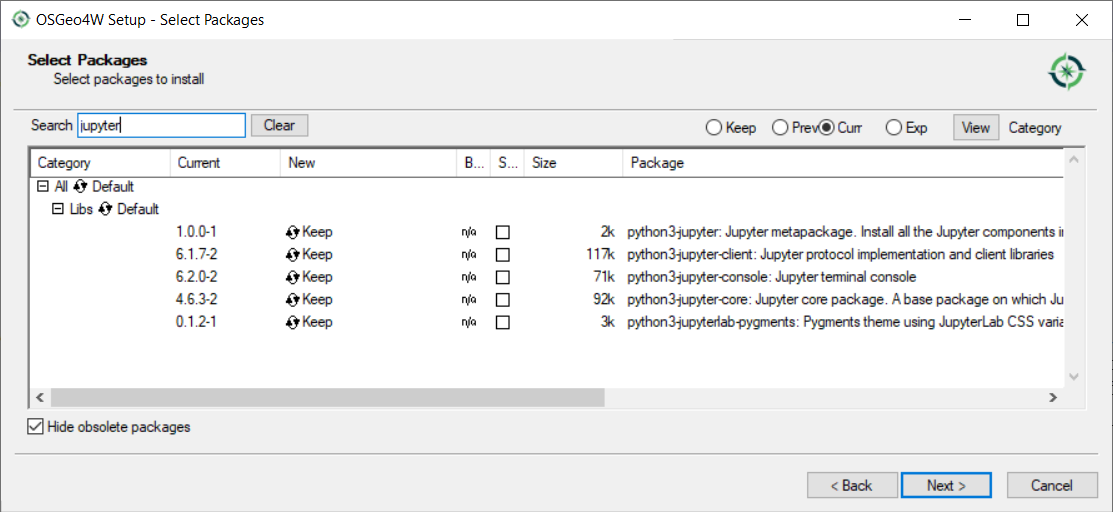
Start the setup from the Start-menu>OSGeo4W, choose the Advanced Install and click forward to the Select Packages-section. Here, search for jupyter and make sure all components are installed (it should say Keep or an installation version number in the New-column). Do the same search for notebook and make sure that it is installed.
Fig. 146 Install of Jupyter components (click on figure for larger image)
If all components are already installed you can cancel your installation, otherwise continue and install.
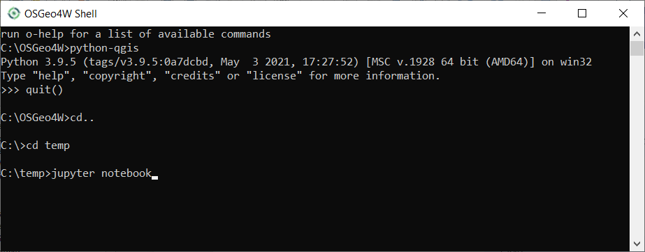
When everything is installed, open the OSGeo4W Shell from the Start-menu. We will use a small work-around to configure our session for UMEP/QGIS scripting. First execute the command python-qgis. This will start a Python session and access the OSGeo and QGIS components needed available for the current shell. Now close this Python session with the command quit(). Now, make use of the cd command to locate yourself in the folder where you have your MyFirstPythopnScript.py-script. If you do not know how to make use of cd-command in dos it is just a google away.
When you are located in the correct folder, type jupyter notebook
Fig. 147 The command to start a Jupyter Notebook (click on figure for larger image)
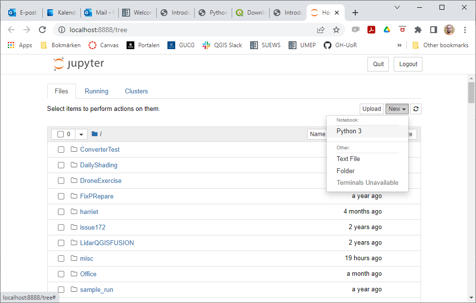
To start a new Notebook click on New and Python3 as shown below.
Fig. 148 Starting a new Notebook (click on figure for larger image)
A Notebook can be executed in so-called cells which give you more control of your code. Start by adding all the lines with your imports from your MyFirstPythopnScript.py-script into the first cell and click Run. A new cell is added below. Now add your saveraster function in the next cell, click Run and then add the code up to the for-loop in a new cell and click Run again. You can restart the code in Kernel>Restart & Clear Output. Here you can also run all cells at the same time (Restart and Run All).
Maybe it is good to save your Notebook at this point. Save as MyFirstNotebookScript. If you check your filesystem you now have a file called MyFirstNotebookScript.ipynd which is the Notebook just created.
Now, in the next cell, add your loop all the way down to the line where you have fillraster = fillraster / index and click Run.
You now see an error that QDate is not found. This is because when you work within a QGIS session, a number of Python libraries are automatically imported. Now we need to import them separately. In your import cell at the top make the following adjustments:
importdatetimefromosgeoimportgdalimportnumpyasnpfromosgeo.gdalconstimport*fromPyQt5.QtCoreimportQDate,QTimeimportsysimportosfromqgis.coreimportQgsApplication# Initiating a QGIS applicationqgishome='C:/OSGeo4W/apps/qgis/'QgsApplication.setPrefixPath(qgishome,True)app=QgsApplication([],False)app.initQgis()sys.path.append(r'C:\OSGeo4W\apps\qgis\python\plugins')sys.path.append(r'C:\Users\__yourusername__\AppData\Roaming\QGIS\QGIS3\profiles\default\python\plugins')importprocessingfromprocessing_umep.processing_umep_providerimportProcessingUMEPProviderumep_provider=ProcessingUMEPProvider()QgsApplication.processingRegistry().addProvider(umep_provider)fromprocessing.core.ProcessingimportProcessingProcessing.initialize()importwarningswarnings.filterwarnings("ignore")
A couple of comments on the code we just adjusted. The sys.path.append-function need to be adjusted to fit your system by changing __yourusername__. The section from import processing access the UMEP algorithms and the import warnings will ignore some warnings that is displayed in the Notebook. If you like to see these warnings, just comment out the two last lines in the cell. IF you want to know how to add QGIS native processing algorithm, see this tutorial.
Now Restart the Kernel and re-run all the cells. you can re-run the cells.
Before we save our fillraster, lets plot the raster in our Notebook, by adding a cell including:
Finally, add the call to the saveraster-function at the end. Now you can play around by changing the start dates and number of days you want to examine.
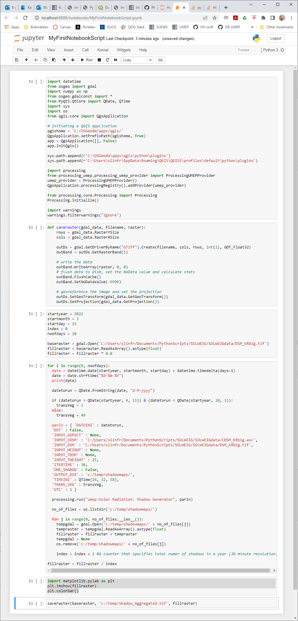
The complete Notebook for this tuorial is shown below:
Fig. 149 The shadow casting Notebook (click on figure for larger image)