Anthropogenic heat - LQF

This tutorial demonstrates how the LQF software is used to simulate anthropogenic heat fluxes (Q_F) for London, UK, in the year 2015, using a mixture of administrative and meteorological data.

Initial Practical steps

UMEP is a python plugin used in conjunction with QGIS. To install the software and the UMEP plugin see the getting started section in the UMEP manual.

For this tutorial you will need certain python libraries: Pandas and NetCDF4. Instructions how to install python libraries are located here.

As UMEP is under constant development, some documentation may be missing and/or there may be instability. Please report any issues or suggestions to our repository.

Data for this exercise

In order to proceed, you will need the zip file named LQF_Inputs_1.zip and a copy of the LQF database. These are available at the following locations:

1. LQF database - v1.2 was used to produce this tutorial

2. LQF input files from the UMEP tutorials data repository.

You may also wish to consult the LQF user guide

The LQF_Inputs_1.zip file contains several datasets to cover all of the tutorials on this page:

• LondonBuildingProfiles.csv: Seasonal diurnal profiles of building energy consumption (1 hour resolution; 7 days; 6 times of year)

• weeklyTraffic.csv: Diurnal profile of road transport volume (1 hour resolution; 7 days)

• DataSources.nml: LQF data sources

• Parameters.nml: LQF Calculation parameters

• griddedResidentialPopulation.*: Spatial data containing residential population counts

• dailyTemperature_2015.csv: Daily mean air temperature in London

LQF Tutorial 1: Simple Q_F modelling

Preparing data

Manage input data files

• Extract the contents of LQF_Inputs_1.zip into a folder on your local machine and note the path to each file (e.g. C:\LQFData\LondonBuildingProfiles.csv)

• Save the LQF database to the same folder as the other data.

Gather information about output areas shapefile

The input data comes with one shapefile (griddedResidentialPopulation.shp) (a collection of files with the same name, one of which ends in .shp). For convenience, the same shapefile is used to define both the model output areas and the residential population density:

• Model output areas: The spatial units where each value of Q_F is calculated.

• Residential population: The number of people within each spatial unit.

LQF needs several pieces of information about the input shapefiles:

1. File path: (e.g. c:\LQFData\PopulationData.shp) - the location of the .shp file on your computer

2. EPSG code: A number that defines the coordinate reference system (CRS) of the shapefile

3. Feature ID field: An attribute within the output areas file that contains a unique identifier for each output area.

4. Start date (population data only): The earliest modelled date for which this dataset should be used

Points (2) and (3) need information from the shapefile itself, as they change depending on the file used. Click here for a guide to finding the EPSG code and feature ID field using QGIS.

Verify the population attribute name

The shapefile used for population data in LQF must always contain an attribute “Pop” that holds the total number of people in that spatial unit. Check this is the case (a similar process to finding the Feature ID field name). The population data was gridded using an algorithm, so the number of people in each area may not be a whole number.

Set up the DataSources.nml file

Add shapefile information

The data sources file needs to be updated so that it can find the various data files, and understands what to do with them. A full description of the Data sources file contents is available here, but this section shows how to build up the entries.

1. Open DataSources.nml using a text editor (we recommend Notepad++) and update the entries according to the information gathered above.

2. There are several sections in the data sources file. Each is bounded by &section_name and ends with “/” and deals with a different part of the input data

3. The “shapefile” entry is the path to the file

4. The epsgCode and featureIds entries are as described earlier

5. The start date for the residential population data is January 1 2011, which needs to be entered as YYYY-mm-dd (2011-01-01).

6. The population shapefile is used for both the output areas and the residential population, so the same filename, EPSG code and featureID are used to describe both of them

The first two sections of the DataSources.nml file should now look like this:

&outputAreas
   shapefile = 'C:/Some/Path/To/Files/griddedResidentialPopulation.shp'
   epsgCode = 32631
   featureIds = 'ID'
/
&residentialPop
   shapefiles = 'C:/Some/Path/To/Files/griddedResidentialPopulation.shp'
   startDates = '2011-01-01'
   epsgCodes = 32631
   featureIds = 'ID'

Add the LQF database and mean daily temperature files

LQF needs to know the location of its database of national parameters.

&database
   path = 'C:/Some/Path/To/Files/LQFDatabase_V1-2.sqlite'
/

• The daily temperature file (dailyTemperature_2015.csv in the zip file) must be formatted appropriately for LQF. See the manual for a detailed description of the file format

&temporal
    ! Air temperature each day for a year
    dailyTemperature = 'C:\Some\Path\To\Files \dailyTemperature_2015.csv'
/

The data sources file should now look similar to the example shown in the LQF manual. In this tutorial, the default diurnal profiles of traffic and building energy use stored in the database will be used, but they can be overridden by adding options to the data sources file.

Run LQF

Under UMEP > Processor > Urban Energy Balance, choose Anthropogenic heat - LQf (LUCY)

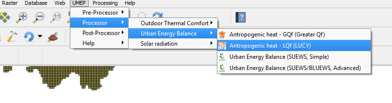
Fig. 50 The location of LQF

This loads the model interface dialog box:

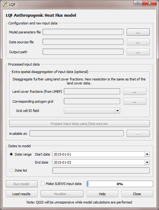
Fig. 51 The dialog for LQF

Choose configuration files and output folder

Working from the top of the dialog box to the bottom…

1. Click the … buttons in the Configuration and raw input data panel to browse to the parameters.nml and DataSources.nml files. A pop-up error message will warn of any problems inside the files.

2. Output path: A folder in which the model outputs will be stored. It is strongly recommended that a new folder is used each time.

3. Extra spatial disaggregation step is not used here

4. Click Prepare input data using Data Sources button. This may be a time-consuming step: It matches each output area with a population and national parameters from the database, which contains different values for each country. If the output areas and population areas are not identical, it also splits the population across output areas based on their overlapping fractions.

5. Once this step is complete, the available at: box will become populated. This folder contains the disaggregated data needed to run the model.

Tip: Save time in future: If the exact same input data files are used in a later study, then the “prepare” step can be skipped: click the “…” button and navigate to a folder that contains the relevant disaggregated data. It will then be copied to the new output folder and used as normal.

Run the model for 1 week

Choose a start date of 11 May 2015, using the start and end date boxes, then select Run.

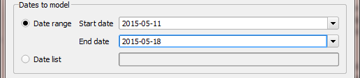
Fig. 52 Setting the start and end date

Visualise results

Once the model run this is finished, press visualise outputs to view some of the model results to open the visualisation tool.

Fig. 53 The visualisation tool in LQF

Create a map of total Q_F at noon

Use the visualisation tool to create a map of all the Q_F components at noon (11:00-12:00 UTC) on May 11 by selecting that time and pressing “Add to canvas”. This may take a moment to process. Close the visualisation tool and return to the main canvas to inspect the four new layers that have appeared.

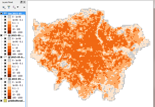
Fig. 54 Example of a map generated with the visualisation tool in LQF

Each layer corresponds to a different Q_F component, Qm (metabolism) and is plotted on the top layer. De-selecting a layer in the Layers panel removes it from view.

Leaving just Q_F (total Q_F) visible, there isn’t much structure in the colours. Add some contrast to it by choosing a different colour scale.

Right-click the Q_F layer, go to Properties > Style, change the colour ramp to “Reds” and choose Mode: Natural Breaks (Jenks). This shows much more structure, although the grid borders are distracting. These can be removed by double-clicking the colour levels and choosing a border colour the same as the fill colour.

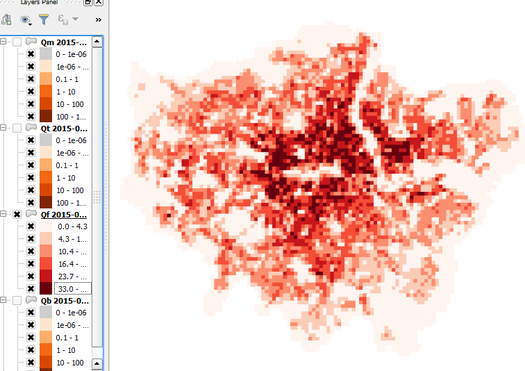
Fig. 55 Same as above but with altered styling

Plot a time series of Q_F in the centre of the city

A time series can be shown for any of the output areas. To identify one of interest, zoom into the city centre, choose the selection tool

Fig. 56 Selection tool in QGIS

and click an output area of interest.

This turns yellow. Right-click it and select the option that comes up.

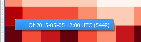
Fig. 57 Information about the output area

then appears on the left, with the ID shown. Make a note of this.

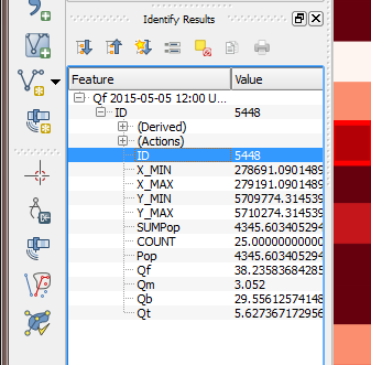
Fig. 58 Information dispalyed from the selected area

Return to the visualisation tool, choose output area 5448 and click show plot. Time series of each Q_F component then appear for the week. Note the lower traffic activity on Saturday and Sunday, and the higher building emissions on Thursday 15th when the weather is colder.

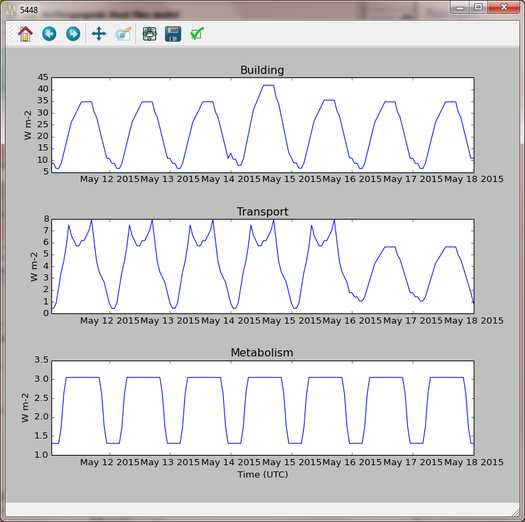
Fig. 59 Temporal plot from the visualisation tool

Recycling of input data

Ideally the model is run only for dates covered by the daily temperature data, but the data is recycled if the model runs beyond the end of the available temperature data. In this tutorial, only 2015 temperatures are provided. If the model ran into 2016, a suitable date from the 2015 temperature data would be selected based on the time of year. Except at the very start or end of the year, the date from 2015 used will be within a few days of the same date in 2016.

Tutorials II: Refining LQF results

Once a basic Q_F estimate has been made (as in the previous section), there are several options to refining this using additional data that may be available.

The following mini-tutorials show how each of these refinements are applied, and the output of the model is compared to that of the standard case.

Tutorial 2a: Custom diurnal profiles

In this scenario, new diurnal profiles for building energy consumption and road vehicle traffic are available for London. These profiles are assumed to better represent the city than the default profiles in the LQF database. In this example, we will re-run LQF using the new profiles.

Each country in the LQF database is associated with two diurnal profiles for transport (a weekend and a weekday version), and the same for building emissions. LQF takes in a week-long profile, starting on Monday, for transport and buildings (shown below), and different profiles can be used for different times of year (click here for full information about diurnal profile files).

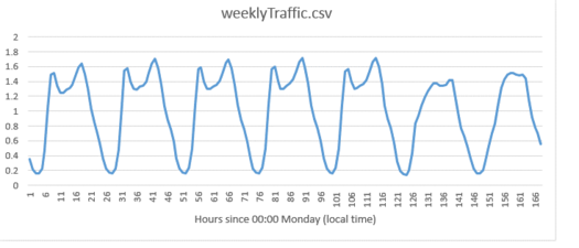
Fig. 60 Custom traffic profile

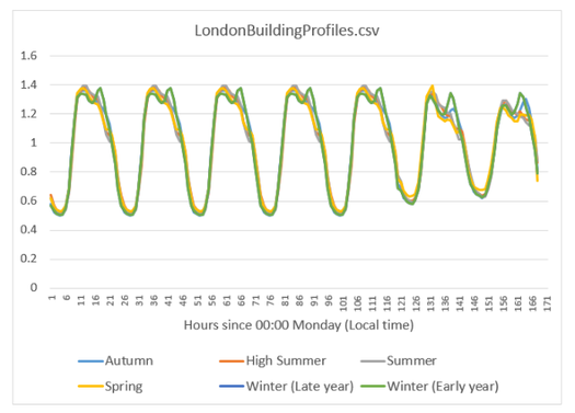
Fig. 61 Custom building profiles

Step 1: Create a duplicate of the DataSources.nml file used earlier

Step 2: create a new folder for the model outputs.

Step 3: Note the paths to the weeklyTraffic.csv and LondonBuildingProfiles.csv files. These contain new profile data

Step 4: Add these to the &temporal section of the new DataSources file using the optional diurnTraffic and diurnEnergy entries. The section should now resemble this:

&temporal
    dailyTemperature = 'C:/Some/Path/To/Files/dailyTemperature_2015.csv'
    diurnTraffic = 'C:/Some/Path/To/Files/weeklyTraffic.csv'
    diurnEnergy = 'C:/Some/Path/To/Files/LondonBuildingProfiles.csv'
/

Step 5: Re-run LQF for 7 days week, starting 11 May 2015, specifying the new DataSources file at run time. Visualising the time series for output area 5448 again:

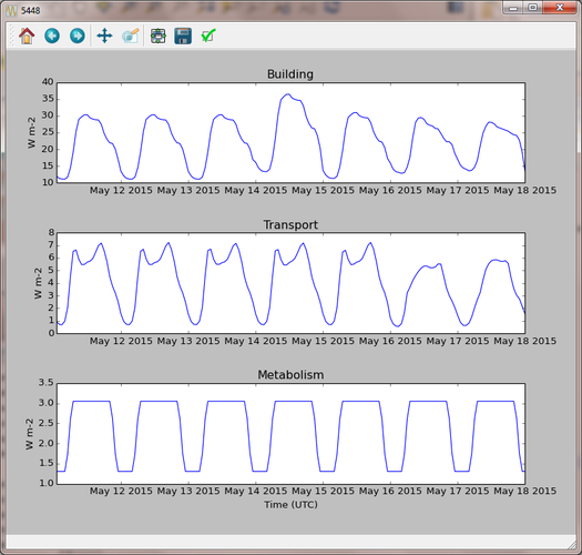
Fig. 62 Output from LQF for seven days in London using cutom profiles

Note how the building and transport emission patterns now change on different days of the week. This is especially noticeable in transport emissions on the final 3 days of the week.

Tutorial 2b: Updating national parameters in the LQF database

LQF takes the latest national attributes (population, vehicle count and energy consumption) up to and including the year(s) modelled. The copy of the LQF database used in this tutorial contains national UK population values in 2010 and 2016. This means the 2010 population is used when 2015 is simulated. This can be updated or added to if data becomes available. The database can be edited using software such as SQLite Browser.

Fictional scenario: The UK population in 2015 was approximate twice that in 2010, but energy consumption remained the same.

Step 1: Make a copy of the LQF database as a backup

Step 2: Open the LQF database in SQLite browser or other suitable software

Step 3: Browse the “attributes” table, which contains national attributes for all countries

Step 4: Locate the population in the UK 2010 row (the value is 62036000.0)

Step 5: Create a new row for the UK in 2015 with the following entries:

Database column	Value
id	United Kingdom
as_of_year	2015
population	120000000
population_datasource	Fake value for test

Step 6: Run the model as in the first example.

Step 7: Visualise the data for output area 5448. Note how the building emissions are approximately half of those in the first example, because the national energy consumption per-capita is now half as much. The vehicle emissions are the same because they are specified per 10,000 people in the LQF database.

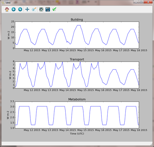
Fig. 63 Output from LQF for seven days in London using cutom database

Step 8: Restore the original LQF database so that the test values do not corrupt future modelling studies.

Tip: To check which national values were used at a given time, check the log folder of the model output directory: NationalParameters.txt contains a list of the values used for each modelled year and country. The following example shows the 2014 value of energy consumption (kwh_year) being looked up for model runs in 2015.

“DB value for United Kingdom kwh_year in modelled year 2015: 966862000000.0 (2014 value)”

See the manual for a list of the parameters stored in the LQF database.

Tutorial 2c: Custom temperature response function

Building emissions are governed by a function that relates the daily mean air temperature to energy consumption. This is a simple treatment that may not capture the full relationship, so a custom function with more parameters can also be used in LQF (full details).

This example shows how to activate the custom temperature response function, and how it affects the results.

The parameters of the custom function are specified using optional entries in the Parameters file. In this example, we will assume that:

• The use of energy stops increasing when the temperature exceeds 20C (weighting is 0.5)

• Energy use increases steeply by 0.5 per degree below 20C

Step 1: Open the parameters.nml file

Step 2: Copy the optional entries needed for the custom temperature response from the manual and ensure the values are consistent with those below

&CustomTemperatureResponse
   Th = 20
   Tc = 20
   Ah = 0.5
   Ac = 0.5
   c = 0.5
   Tmax = 50
   Tmin = -10
/

Step 3 : Save the parameters file and run the model as in the original tutorial. Note how the day-to-day variations in the building emissions are much greater than in Tutorial 1, but the transport and metabolism emissions remains the same as before.

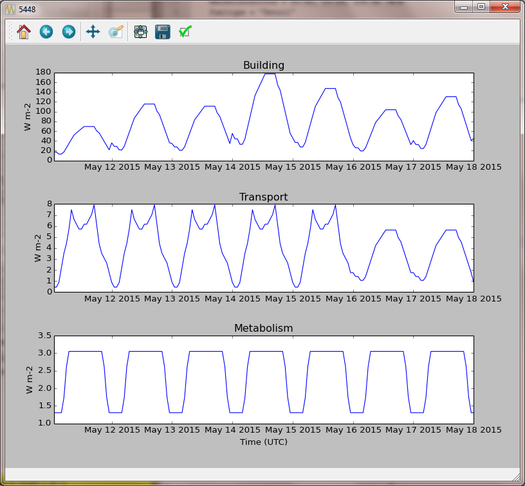
Fig. 64 Output from LQF for seven days in London

Tutorial finished.