In this tutorial you will show you how to produce maps of thermal comfort indices using outputs from two different models in UMEP.
The two different models used are SOLWEIG (radiation model) and URock (wind model). These two models are combined in the SpatialTC-tool to generate raster maps on thermal indices such as PET, UTCI and COMFA. This tutorial will make use of PET (Physilogical Equivalent Temperature) as an example.
The UMEP tutorial datasets can be downloaded from our here repository
here.
Download, extract and add the raster layers (DSM, CDSM, DEM), the building polygon layer and the line profile layer (not used in this tutorial) into a new QGIS session. Coordinate system of the grids is Sweref99 TM (EPSG:3006).
The output data generated from the introduction tutorial on Urock will be used for this exercise. If you have not gone through Urban Wind Field - Introduction to URock, do so and make sure that you produce data with vegetation information included (last section of the tutorial).
It is recommend to get familiar with the SOLWEIG model before you produce your input for SpatialTC by looking at Thermal Comfort - Introduction to SOLWEIG but below you will also find instructions on how to generate the data needed. All tools should be executed via UMEP for Processing.
Some additional data has to be prepared in order to execute the SOLWEIG-model.
To run SOLWEIG various sky view factor (SVF) maps for both
vegetation and buildings must be created (see Lindberg and
Grimmond
(2011)
for details).
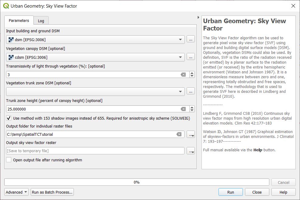
You can create all SVFs needed (vegetation and buildings) at the
same time. Use the settings as shown below. Use an appropriate
output folder for your computer.
Fig. 119 Settings for the SkyViewFactorCalculator.
If you look in your output folder you will find a zip-file and a .npz-file containing all the
necessary SVF maps needed to run the SOLWEIG-model.
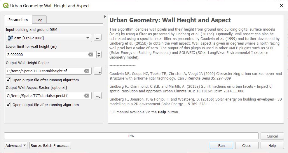
Another pre-processing plugin is needed to create the building wall heights and aspect. Open UMEP -> Pre-Processor -> Urban geometry -> Wall height and aspect and use the settings as shown below. QGIS scales the loaded rasters by a cumulative count out approach (98%). As the height and aspect layers are filled with zeros where no wall are present it might appear as if there is no walls identified. Rescale your results to see the walls identified (Layer Properties > Symbology).
Fig. 120 Settings for the Wall height and aspect plugin.
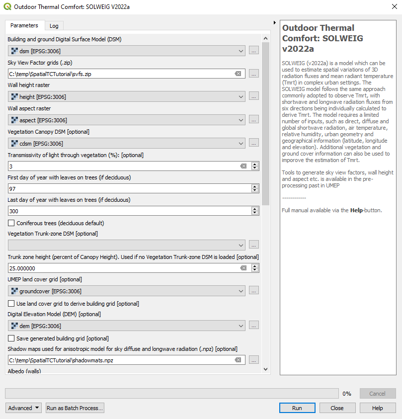
Open the SOLWEIG plugin and use the settings shown below (see both figures). Do not
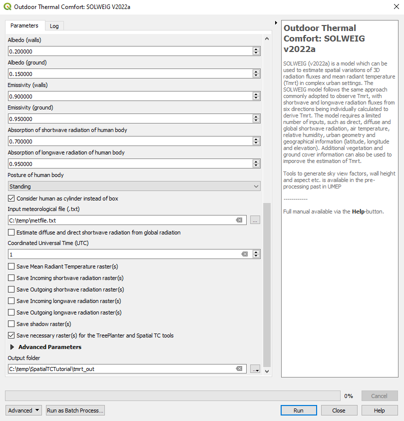
forget to tick Save necessary raster(s) for the TreePlanter and Spatial TC tools. The metfile is found in the downloaded tutorial data (metfile.txt) and is a clear (and not very warm) Summer day. Click Run.
Fig. 121 The settings for your SOLWEIG run (click on figure for larger image).
Fig. 122 Continuing.. The settings for your SOLWEIG run (click on figure for larger image).
Details of the model inputs and outputs are provided in the SOLWEIG manual. As the focus of this tutorial is to run SpatialTC, only the most critical parameters are used. Many other parameters can be modified to more appropriate values, if applicable.
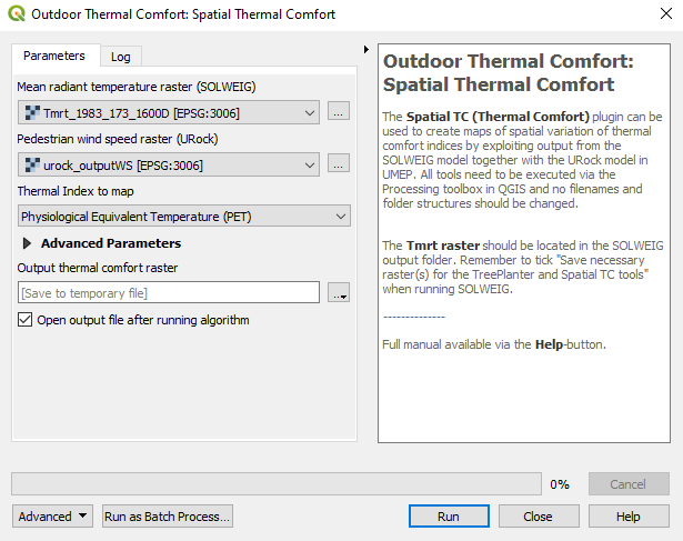
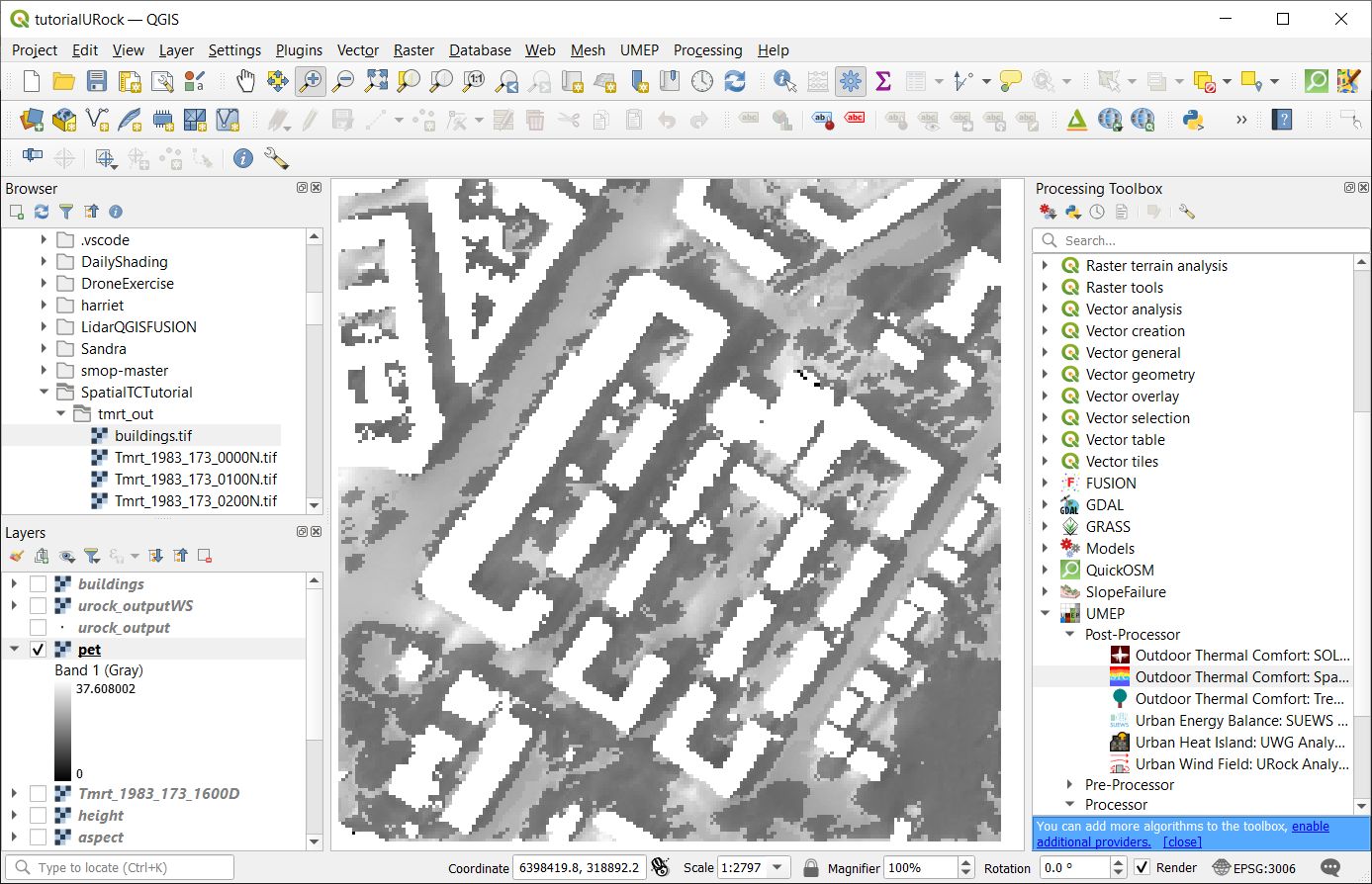
Now you will run SpatialTC based on the output from the SOLWEIG and URock run in the previous sections.
You need to specify two rasters: one of the mean radiant temperature that has been produced by SOLWEIG and one with the pedestrian wind speed produced by URock.
Load the Tmrt_1983_173_1600D.tif into your QGIS project. This file can be found in your outout folder form the previous SOLWEG-run. Do not change the file name as the info in the name will be used to identify the meteorological information that is needed to calcualte PET.
Last you need to select the thermal comfort index to map (PET for this tutorial). The Advanced parameters describing the person to consider for the comfort index can also be defined but the default values are kept for this tutorial. Then click Run.