Spatial data - Generating UMEP input data from a LiDAR point cloud

Note

This tutorial is making use of FUSION/LDV which makes it restricted to Windows OS only.

The purpose of this tutorial is to create spatial input data for UMEP and get familiar with some of the various tools available in QGIS concerning processing of data obtained by the airborne LiDAR technology.

You will get acquainted with FUSION/LDV, a so-called free software (not to be confused with open source) developed to process point clouds. The exercise focuses on the city and how to make use of LiDAR data in urban environments.

The exercise is divided in two parts:

1. In the first part you will get acquainted with some different features that are available in QGIS and how to use other open source software within QGIS. You will also learn how to use FUSION effectively using the Windows Command Prompt. The end products will be a DSM and CDSM. This part of the tutorial is losely based upon the method presented in Lindberg and Grimmond (2011).

2. In the second part, you will create a basic land cover data using QGIS/FUSION. This part of the tutorial is losely based upon the method presented in Hedblom et al. (2017).

PART 1 - Creating DSM and CDSM

QGIS graphical interfaces and settings

In this exercise, you will work with an area around Earth Science Center in Gothenburg, Sweden. The dataset consists of a number of vector layers from Lantmäteriets (Swedish Cadastral and Mapping Authority) Fastighetskarta and a laser point cloud derived from the National Elevation Model (NH) in Sweden.

In this exercise you will make use of the Processing Toolbox (right side of Figure 1) where many of the geoprocessing algorithms are found, both from the QGIS core and from other open source software and libraries such as GDAL, GRASS, SAGA GIS, R, FUSION, UMEP etc. If the toolbox is unavailable, go to Processing and click on Toolbox.

Next step is to download and activate the plugin that makes it possible to use the FUSION software within QGIS3.

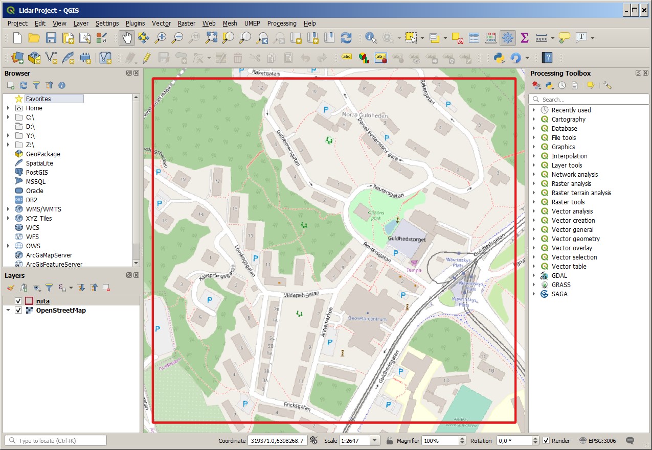
Fig. 84 Figure 1. The Graphical User interface for QGIS 3.6. The open street map is retrieved from the OpenLayers plugin.

FUSION is a freeware (Free Software) without restrictions, developed especially for using LiDAR technology in forestry, but it can also be used in other applications. FUSION can be downloaded from http://forsys.sefs.uw.edu/fusion/fusionlatest.html. Make sure that FUSION is installed at C:\FUSION. If not, locate the FUSION folder and remember its location. Now go to Plugins > Manage and Install Plugins, search for FUSION, click on FUSION for Processing and click Install Plugin. This is a processing plugin porting many of the FUSION tools directly into the QGIS processing framework.

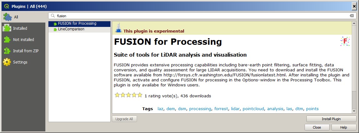
Fig. 85 Figure 2. The Plugin Manager in QGIS 3.6.

To make use of FUSION inside QGIS you have to configure some initial settings. In the Processing Toolbox, click on the monkey wrench (Options) and configure FUSION as shown in Figure 3. Remember to point to the directory where FUSION is installed on your system. If successful, a FUISON-menu should have appeared in the Processing toolbox.

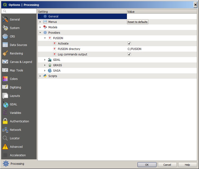
Fig. 86 Figure 3. Settings to activate FUSION for processing in QGIS 3.6

Get started with FUSION

Start by examining the point cloud that you will make use of for the rest of this exercise. The data can be downloaded from here (link also at end of this document). All data is projected in SWEREF99 TM (EPSG:3006) so it is very important to specify this when you add your data into QGIS. Save the data in a location where you have rights to read and write, e.g. the Desktop or a USB-stick. In the Processing Toolbox go to FUSION > Visualisation > Open viewer and open gvc.las. Examine your point cloud. Make use of the help (?) button to find out which classes are within this particular point cloud. As you will discover, this is a very basic point cloud including only two classes (ground and unclassified).

Expand FUSION in the Processing Toolbox. Here you will find a number of FUSION algorithms, divided up into different categories. This is far from all that FUSION can do. The full manual of FUSION is available from: http://forsys.cfr.washington.edu/Software/FUSION/FUSION_manual.pdf. In this document you can find specification on all the algorithms available in FUSION. We will also look at how to use the algorithms that are not available from within the graphical interface of QGIS.

As the ground points were already classified in the point cloud, you can now generate a digital elevation model. If the point cloud would have been unclassified, you could have exploited the Ground Filter to filter out ground points. Open FUSION > Surface > Grid Surface Create and configure the following settings (Figure 4), before clicking Run. Remember to save your data at an location where you have read and write access on your system.

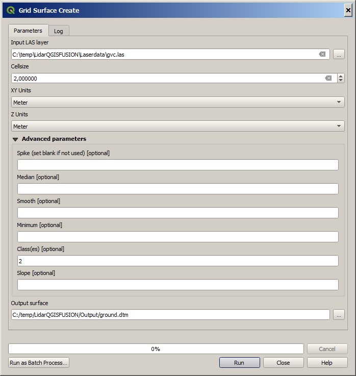
Fig. 87 Figure 4. Setting for Grid Surface Create when creating a DEM.

For all the elevation models that we create in connection with this exercise, we will use the 2-meter resolution as this is what the point cloud is originally designed for. Grid Create Surface can only save so-called .dtm-files, which is a in-house file format in FUISON. This file cannot be opened in QGIS but we can study our soil model using FUSION LAS viewer (Figure 5).

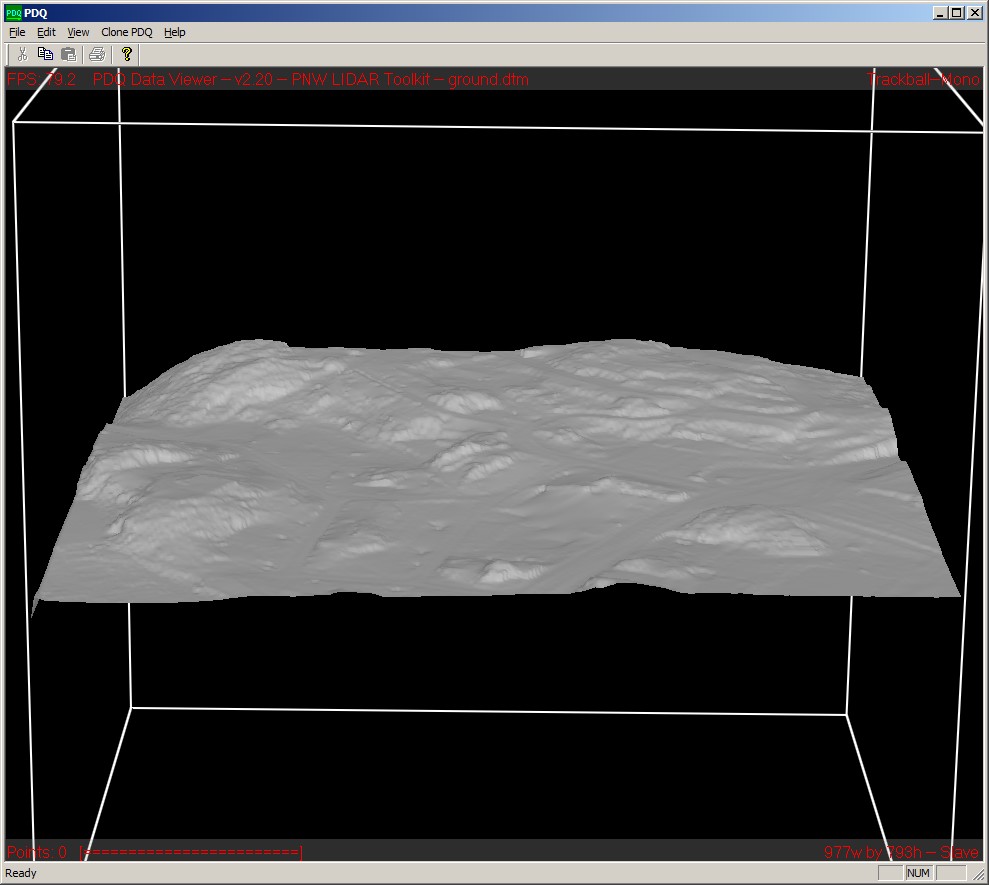
Fig. 88 Figure 5. Ground.dtm.

As you can see there are a variety of settings to configure in Grid Surface Create. To see what they all do, you can study FUSION Manual. To create a geoTIFF grid from your .dtm file we will use a FUSION algorithm outside of QGIS. This method is important to be familiar with when you want to use FUSION for other purposes, such as creating automated scripts etc, later on. Therefore, it is very useful to learn how to make use of the FUSION algorithms from the Windows Command Prompt.

Go to the Start menu in Windows and open the Command Prompt (you can search for cmd if you cannot find it). For those of you who are beginners in dos syntax you only need one command for this exercise (cd). This command allows you to move between folders. Typing cd.. you can move backwards in the folder structure. When you are at the system root, type cd C:\FUSION. To see what’s in the folder, you can write the dir (Figure 6).

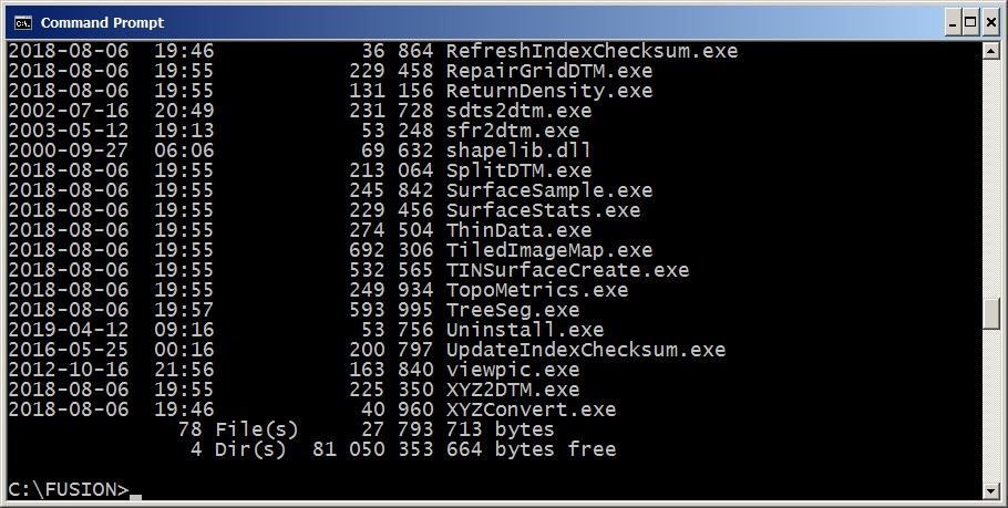
Fig. 89 Figure 6. The Windows Command Prompt

Now use the cd-command to locate the folder where you saved ground.dtm. You must also make the command prompt “aware” of where the FUSION algorithms are located. Type the command as shown in Figure 7 (path %PATH%;C:\FUSION).

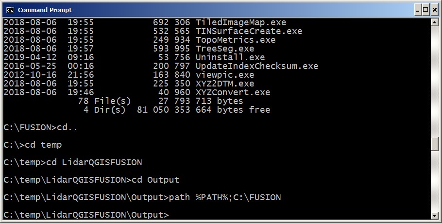
Fig. 90 Figure 7. Adding an environment path in the command prompt.

Now you can use all the executable algorithms that are available in the C:\FUSION\. Try by typing gridsurfacecreate. Now you will see the documentation available for this specific algorithm. As you want to convert your .dtm file you will make use of DTM2ASCII. Type the following command:

dtm2ascii /raster ground.dtm

You have now created an ESRI ASCII grid (in the same folder as ground.dtm) that you now can open QGIS. Open ground.asc in QGIS. You can also open the building footprint polygons from Fastighetskartan (by_get.shp). Do not close the Command Prompt. If you have already done this, you need set your path to Fusion again.

Create Digital Surface Models using QGIS/FUSION

A Digital Surface Model (DSM) is an elevation model that contains the heights of objects (such as building heights). Usually, ground elevation is also included. A model containing only ground level elevation is usually defined as a Digital Elevation Model (DEM). There are several ways to create a DSM. First, you should make use of an additional algorithm from the command prompt, PolyClipData. The algorithm is used to separate out certain points from the point cloud. Remove by_get.shp from your QGIS project if the layer is loaded. Locate yourself in the LaserData folder and enter the following command in one line:

polyclipdata /outside /class:1 “c:\temp\LidarQGISFUSION\Fastighetskartan\by_get.shp” “c:\temp\LidarQGISFUSION\Output\veg.las” “gvc.las”

Sometimes the folder paths malfunction. If you get an error message, try copying the by_get.shp in the same folder as gvc.las and then remove the path from the command. Remember that a shape file consists of many files, i.e. you need to copy all files starting with the name by_get. What you did with the above command was take all the points classified as unclassified, with the switch /class:1, and cut them based on the building footprints with the switch /outside. Examine the results in the FUSION LAS viewer.

Run the same algorithm, but just cut the points that are within the building footprints by removing the /outside-switch. Name the output buildings.las.

Finally, cut out all the ground points. Name the output ground.las. If you are not able to write the correct syntax, see the solutions at the end of this exercise.

Now let us create a DSM that includes both land and building heights. We do this, use Processing Toolbox > FUSION > Surface > Canopy Model as shown in Figure 8. In this algorithm we can use the switch /ascii and thereby avoid creating an ESRI ASCII grid afterwards. Instead, an ascii grid with the same name as your .dtm file is now created. Note that two las files are added as input layers.

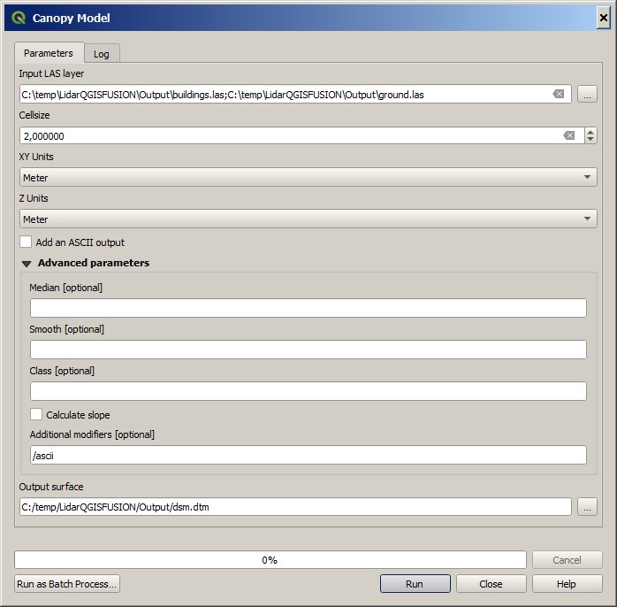
Fig. 91 Figure 8. Settings in Canopy Model in order to create a building and ground DSM.

If you are successful, DSM.dtm should look like Figure 9.

An asci file has also been created (DSM.asc). This is a very simple raster file format and cannot be e.g. embedded with coordinate system information. Therefore we need to convert it into another format, e.g. geoTIFF. Open DSM.asc in QGIS and create a geotiff copy by right-clicking and choosing Export > Save as…. Save the GeoTIFF in the Output folder and name it DSMtif.tif. Keep all other settings as standard.

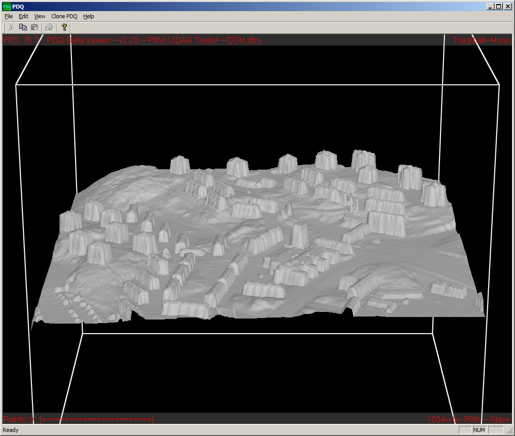
Fig. 92 Figure 9. DSM.dtm.

We will also try to create a DSM which contains only vegetation (trees and shrubs). This requires some additional steps and to achieve the best possible results, one needs to undergo a number of filtering processes. You can study this further in Lindberg and Grimmond (2011). To create a decent vegetation model, we will use two types of filters. First, we want to filter out lower points that can be, for example, people or cars. To do this, we use ClipData. Unfortunately there is a bug in the algorithm of running it from the Processing Toolbox so we need to run it from the command prompt. Locate your folder Output and enter the following:

clipdata /ground:ground.dtm /zmin:2.5 veg.las veg_filt.las 318864.0 319364.0 6397926.0 6398400.0

This was done to exclude all the points that are lower than 2.5 meters from our ground model (/zmin:2.5). The coordinates at the end are taken from the extents parameters in DSM.asc.

Now you can run the Canopy Model again with settings according to Figure 10.

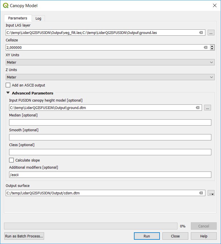
Fig. 93 Figure 10. Settings in Canopy Model in order to create a vegetation DSM.

Adding ground.dtm as Input Ground DTM layer normalizes all values ​​to be meters above ground level instead of meters above the sea level. Open cdsm.asc in QGIS. As you can see, you need to perform some additional steps before you can be satisfied. The trees have a lot of “holes”, there are also occasional lamp posts, etc. Plus the buildings in the model are visible. This depends on how the CanopyModel algorithm works. You can read more about this in the manual if you are interested. Let’s start by removing buildings. To do this, create a new polygon layer by buffering the building footprint layer (by_get.shp) by 2 meters (Vector > Geoprocessing Tools > Buffer). Set End cap style to Flat and Join style to Miter. Name your new shapefile by_buff.shp and save it in the folder Fastighetskartan. We must also create an additional attribute for by_buff.shp with the value 0. Open the attribute table and then the Field Calculator (abacus). Configure the following settings (Figure 11) and click OK. Then save and close the editor mode (buttons to the top left of the attribute table).

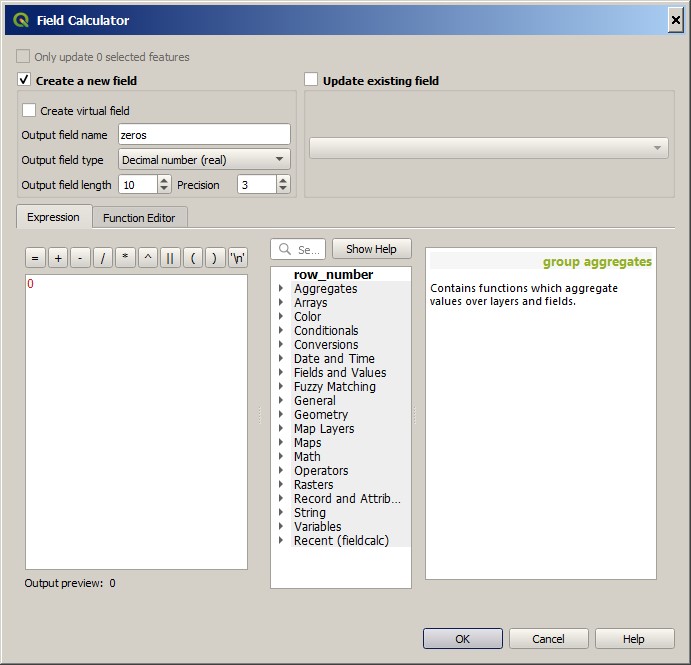
Fig. 94 Figure 11. How to add a new attribute column containing only zeros.

Now go to the Raster -> Conversion -> Rasterize and configure the following settings as in Figure 12. The Output extent is taken from the dsmtif.tif layer.

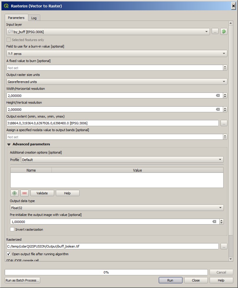
Fig. 95 Figure 12. Rasterize in QGIS.

Open the Raster Calculator and multiply buff_bolean with cdsm. Call the new layer cdsm_filt.tif. This operation has now removed vegetation pixels that were present within the buffered buildings.

Unfortunately, the Canopy Model algorithm in FUSION/QGIS is produces very small elevations when it is normalized against the ground.dtm. Therefore, we need to remove these values from the vegetation raster. This can be done in the Raster Calculator in QGIS. Open Raster Calculator and choose write the following expression in the Raster Calculator Expression Window:

(cdsm_filt@1 > 0.5) * cdsm_filt@1

Call the output file cdsm_filt2.tif and save as a geoTIFF.

Finally, you need to run a majority filter to remove some noise (posts, etc.) on our vegetation DSM. A majority filter replaces individual pixels that are surrounded by pixels with the same value. In our case, for example, a positive pole height value is surrounded by ground pixels (zeros). This replaces the pixel value to the value that occurs most in the filter window (usually 3x3), i.e. zero. Search for Majority filter from SAGA GIS in the Processing Toolbox. Run the filter algorithm using default settings except changing the Theshold values to 65. Use a temporary output and then export the layer as a geoTIFF with the name cdsm_final. There are also other filters that you could make use of. For example, filters to fill gaps in the vegetation or remove linear features (see Linberg and Grimmond 2011). If you feel you have much time left, consider how to fill gaps in vegetation using filtering techniques.

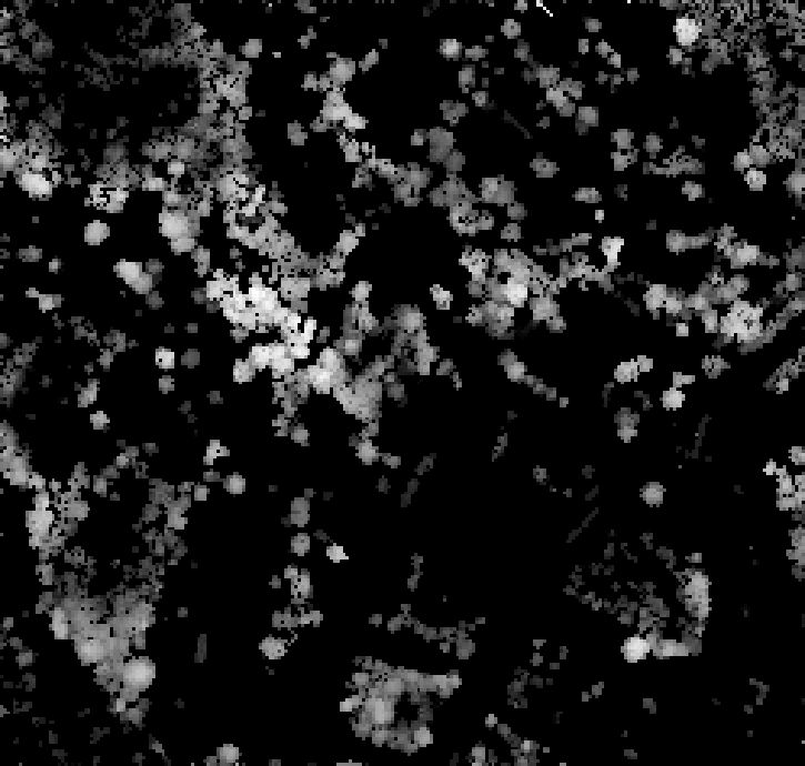
Fig. 96 Figure 13. cdsm_final.tif

PART 2 - Land Cover data

The land cover in UMEP consists of seven classes (buildings, paved, deciduous trees, conifer trees, bare soil and water). This part of the exersice you will make use of the data produced in Part 1. You will try to derive as many classes as possible.

Buildings and paved

First you need to create a new boolean raster using your building polygon layer. Create a new attribute called zeros in by_get and re-run Rasterize as in figure 12 but now use by_get as the input layer and build_bolean.tif as output (Rasterized).

Deciduous trees

Now create a boolean raster where vegetation = 1 and ground = 0 in the Raster Calculator. Call the new layer veg_bolean.tif (“cdsm_final@1” > 0). We will not try to separate deciduous and confier here.

Grass

Now open ground.las in the FUSION viewer and color point using intensity data (press the N key). As shown in Figure 14, each laser pulse returns to the reciever with an intensity. As the laser pulse usually is within the red spectrum, features such as grass (vegetation) has a high intensity and can therefore be identified (Figure 14).

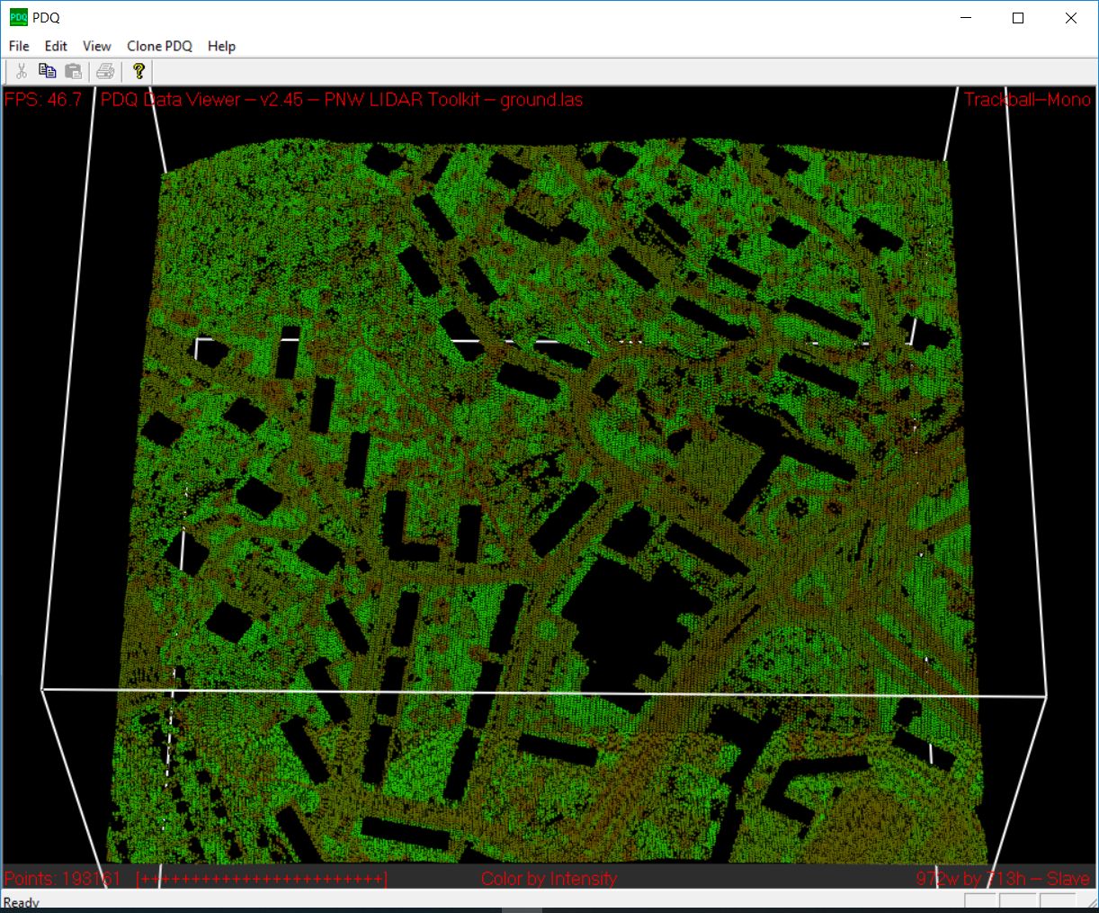
Fig. 97 Figure 14. Ground.las visulized based on intensity values.

Open Point cloud analysis > Intensity Image in FUSION and configure the settings as in Figure 15.

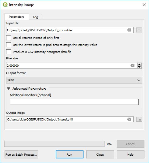
Fig. 98 Figure 15. Settings for the Intesity Image tool.

This creates a 3 band raster image. You need to add it to your project (Intensity.bmp). One simple way to reduce it to only one layer is to use the Raster Calulator and only save one of the band. Call the output Intensity1.tif. Buildings and other NoData-features are here classified as 255. Reduce these values to zeros using the Raster Calculator again ((“Intensity1@1” < 255) * “Intensity1@1”). Call the output layer Intensity1nodata.tif. Now try to find a suitable threshold value that can represent the lower value of grass. This can be done by either identifying values using the Identify tool (i with a mouse pointer) or you can try to visulize the grass in the Symbology tab under Properties. This requires some knowledge of the area (i.e. what is grass and what is not) or you can make use of e.g. QuickMapServices-plugin and overlay i.e. Google satellite images. When satisfied (I used >125) create a boolean image where grass has the value 1 and other surfaces 0, using the Raster Calculator. Call the layer lc_bolean.tif.

Bare soil and water

This is about as far as you can come with a point cloud like this. Bare soil is actually not present within this domain and water usually has no returns back and can therefore be hard to classify. There are techniques to do so, but not within the scope of this tutorial. One possibility is to use a vector dataset (e.g. Figure 1) and extract e.g. water from that dataset and incorporate into the land cover data. Another would be to exploit the fact that lidar returns are almost absent from water bodies (lakes, ponds etc.). You can examine gvc.las in the FUSION viewer and spot a small pond in the center of the study area. However, you will also see other areas with no returns, e.g. metal roofs etc. This makes deriving water bodies a bit of a challenge, but not impossible. You can use e.g. r.null in the processing toolbox to try to derive water.

Merging into on land cover grid

Make use of the Raster Calculator again using the following syntax:

("build_bolean@1") + ("lc_bolean@1" * 2) + (("build_bolean@1" * "veg_bolean@1") * 3)

Call the output landcover_raw.tif.

Finally, you need to appoint the correct values to the different classes. That can be done using UMEP > Pre-Processor > Urban Land Cover > Land Cover Reclassifier. You can qualitatively check your land cover classification against satellite imagery, such as the Google Satellite in QuickMapServices.

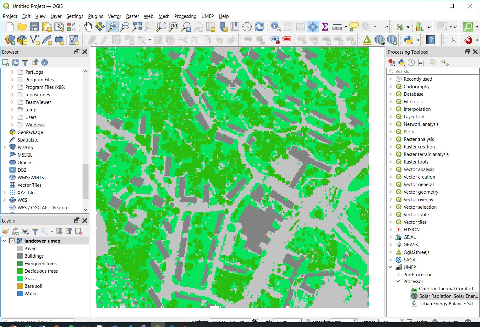
Fig. 99 Figure 16. The land cover maps produced from the lidar point cloud.

Tutorial finished.

Commands

To add an environment path in the command prompt:

Path %PATH%;C:\\FUSION

To cut out laser points within building footprints:

polyclipdata /class:1 ”c:\LidarQGISFUSION\Fastighetskartan\by_get.shp” ”buildings.las” ”gvc.las”

To cut out laser points on the ground:

C:\LidarQGISFUSION\Laserdata>polyclipdata /outside /class:2 ”c:\LidarQGISFUSION\Fastighetskartan\by_get.shp” ”ground.las” ”gvc.las”

References

Hedblom, M., Lindberg, F., Vogel, E., Wissman, J. and Ahrné, K. (2017) Estimating urban lawn cover in space and time: case studies in three Swedish cities. Urban Ecosystem. 20: 1109-1119..

Lindberg, F. and Grimmond, C. (2011) Nature of vegetation and building morphology characteristics across a city: Influence on shadow patterns and mean radiant temperatures in London. Urban Ecosystems 14:4, 617-634.

Link to data: https://github.com/Urban-Meteorology-Reading/Urban-Meteorology-Reading.github.io/blob/master/other%20files/LidarQGISFUSION.zip