Footprint modelling
Introduction
Each meteorological instrument has a ‘source area’ (sometimes referred to as footprint), the area that influences the measurement. The shape and location of that area is a function of the meteorological variable the sensor measures and the method of operation of the sensor.
For turbulent heat fluxes measured with a sonic anemometer, extensive effort has been directed to try and model the ‘probable source area location’ (Leclerc and Foken 2014). Numerous models exist, but the Kormann and Meixner (2001) and Kljun et al. (2015) models are used in UMEP. Both models require input of information about the wind direction, stability, turbulence characteristics (friction velocity, variance of the lateral or crosswind wind velocity) and roughness parameters. Kljun et al. (2015) requires the boundary layer height.
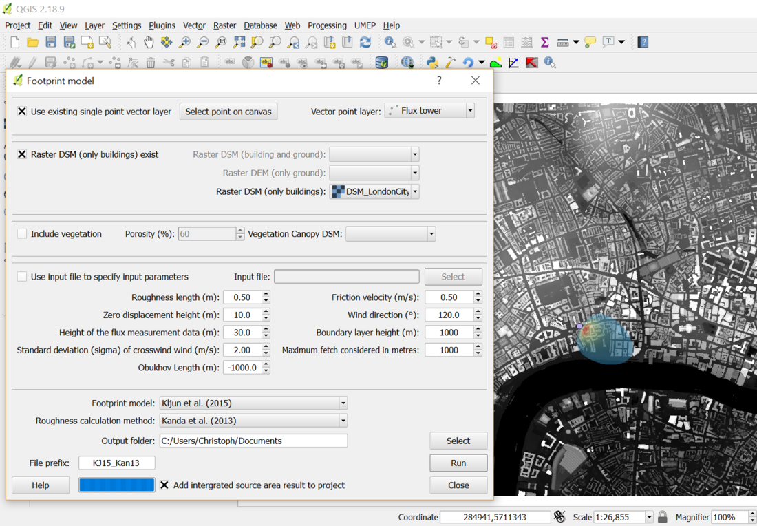
Fig. 13 Example result (example from older version). Click on figure for larger image.
Initial Practical steps
If QGIS is not on your computer you will need to install it.
Then install the UMEP plugin.
Start the QGIS software
If not visible on the desktop use the Start button to find the software (i.e. Find QGIS under your applications). Use QGIS3.
When you open it on the top toolbar you will see UMEP.
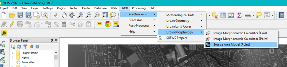
Fig. 14 Location of footprint plugin (click on figure for larger image)
If UMEP is not on your machine, add the UMEP plugin by go to Plugins>Manage and Install Plugins in QGIS and search for UMEP. Click Install plugin. Here you can also see if there is newer versions of your added plugins.
Preferably, read through the section in the online manual BEFORE using the model, so you are familiar with it’s operation and terminology used.
Data for Tutorial
Use the appropriate data:
Prior to Starting
Download the Data needed for the Tutorial. You can use either the Reading or the London dataset.
Load the Raster data (DEM, DSM, CDSM) Note: a CDSM exists for London but not for Reading
Go to: Layer > Add layer > Add Raster Layer. Locate downloaded files add add them to your QGIS project.
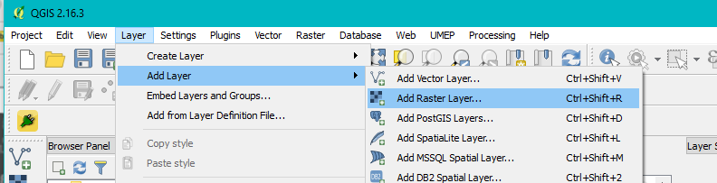
Fig. 15 Loading a raster layer to QGIS (click on figure for larger image)
Have a look at the layers (see lower left) - if you untick the box layer names from the top you can see the different layers.
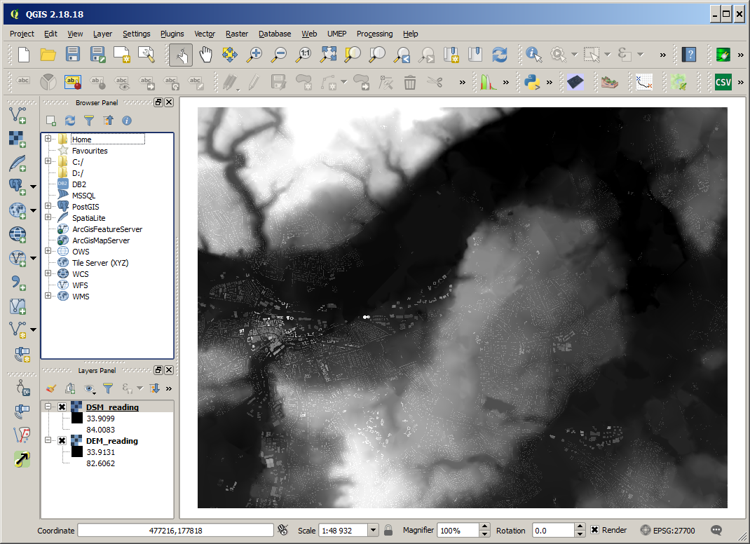
Fig. 16 The Reading data loaded into QGIS (click on figure for larger image)
Source Area Modelling
To access the Source area (Footprint) model, go to UMEP -> Pre-processor > Urban Morphology > Source Area Model (Point).
Click on Select Point on Canvas – then select a point (e.g. where an Eddy Covariance (EC) tower site is located)
Select the appropriate surface elevation data file names
Choose the model you wish to run (Kormann and Meixner 2001 or Kljun et al. 2015)
Some initial parameter values are given - think about what would be appropriate values for your site and period of interest. The manual has more information (e.g. definitions) of the input variables.
The values are dependent on the meteorological conditions and the surface surrounding the site. The former obviously vary on an hour to hour basis (or shorter time periods), whereas the others are dependent on the wind direction and the fetch characteristics.
Add a prefix and an output folder.
Tick “add the integrated source area to your project”. This will provide visual information of the location of the source area (footprint)
Click Run. If you get an error/warning message (model is unable to execute your request, as the maximum fetch exceeds the extent of your grid for your point of interest. Measure the distance to the limit of your raster maps
To allow the model to work for the dataset with your point of interest you need to adjust the maximum fetch distance.
In the QGIS toolbar, locate the Measure tool (Ruler or Ctrl + Shift + M).
Measure the distance to the point of interest to the nearest boundary of the DSM data set.
Adjust the maximum fetch accordingly.
Click Run and wait for the calculations to finish.
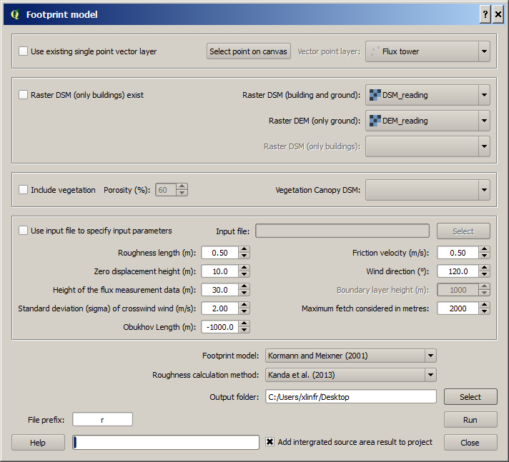
Fig. 17 Snapshot of the Footprint plugin using Reading data (click on figure for larger image)
The output is a source area grid showing the cumulative percentage of source area influencing the flux at the point of interest.
The other output is a text file giving both the input setting variables and the output morphometric parameters calculated based on the source area generated. More information is provided in the manual, row titled: “Output”
It is possible to input a text file to generate a source area based on morphometric parameters (e.g. an hourly dataset). However, for now you can modify the input variables set in the interface. The format of such a file is given in the manual.
Iterative process
To work with a site with no morphometric values known a priori.
Use the MorphometricCalculator(Point) tool in the UMEP plugin to select a point to get the initial parameter values:
UMEP-> Pre-Processor -> Urban Morphology -> Image Morphometric Calculator (Point)
Open the output files
Anisotropic file – has the values in each sector that you selected. This is appropriate if the area is very inhomogeneous.
Isotropic file - has the average value for the area
Use these values to populate the source area model window.
Tutorial finished.
Roughness parameters
In the UMEP plugin the roughness length and zero plane displacement length can be calculated with a morphometric method based on the Rule of Thumb (Grimmond and Oke 1999) as the default. There are other methods available: Bottema (1995), Kanda et al. (2013), Macdonald et al. (1998), Millward-Hopkins et al. (2011) and Raupach (1994, 1995). Many of these have been developed for urban roughness elements. The Raupach method was originally intended for forested areas but has also been found to perform well for urban areas.
With wind profile and eddy covariance anemometric data and the source area model, appropriate parameters can be determined and morphometric methods assessed (e.g. Kent et al. 2017).
References
Bottema M 1995: Parameterisation of aerodynamic roughness parameters in relation to air pollutant removal ef?ciency of streets. Air Pollution Engineering and Management, H. Power et al., Eds., Computational Mechanics, 235–242.
Grimmond CSB and TR Oke 1999: Aerodynamic properties of urban areas derived, from analysis of surface form. Journal of Applied Climatology 38:9, 1262-1292
Kanda M, Inagaki A, Miyamoto T, Gryschka M, Raasch S 2013: A new aerodynamic parameterization for real urban surfaces. Boundary- Layer Meteorol 148:357–377. doi:10.1007/s10546-013-9818-x
Kent CW, Grimmond CSB, Barlow J, Gatey D, Kotthaus S, Lindberg F, Halios CH 2017: Evaluation of Urban Local-Scale Aerodynamic Parameters: Implications for the Vertical Profile of Wind Speed and for Source Areas. Boundary-Layer Meteorol 164:183-213.
Kljun N, Calanca P, Rotach MW, Schmid HP 2015: A simple two-dimensional parameterisation for Flux Footprint Prediction (FFP). Geoscientific Model Development.8(11):3695-713.
Kormann R, Meixner FX 2001: An analytical footprint model for non-neutral stratification. Bound.-Layer Meteorol., 99, 207–224 http://www.sciencedirect.com/science/article/pii/S2212095513000497#b0145
Kotthaus S and Grimmond CSB 2014: Energy exchange in a dense urban environment – Part II: Impact of spatial heterogeneity of the surface. Urban Climate 10, 281–307 http://www.sciencedirect.com/science/article/pii/S2212095513000497
Leclerc MY and Foken TK 2014: Footprints in Micrometeorology and Ecology. Springer, xix, 239 p. E-book
Macdonald, R. W., R. F. Griffiths, and D. J. Hall, 1998: An improved method for estimation of surface roughness of obstacle arrays. Atmos. Environ., 32, 1857–1864
Millward-Hopkins JT, Tomlin AS, Ma L, Ingham D, Pourkashanian M 2011: Estimating aerodynamic parameters of urban-like surfaces with heterogeneous building heights. Boundary-Layer Meteorol 141:443–465. doi:10.1007/s10546-011-9640-2
Raupach MR 1994: Simpli?ed expressions for vegetation roughness length and zero-plane displacement as functions of canopy height and area index. Bound.-Layer Meteor., 71, 211–216. doi:10.1007/BF0070922
Raupach MR 1995: Corrigenda. Bound.-Layer Meteor., 76, 303–304.
Contributors to the material covered
University of Reading: Christoph Kent, Simone Kotthaus, Sue Grimmond University of Gothenburg: Fredrik Lindberg Background work also comes from: UBC (Andreas Christen); Germany: Kormann and Meixner (2001); Japan: Kanda et al. (2013); UK: Millward-Hopkins et al. (2011), Macdonald et al. (1998); Australia: Raupach (1994, 1995); Netherlands: Bottema (1995)
Authors of this document: Kent, Grimmond (2016). Lindberg