In this tutorial you will use a model SOlar and LongWave Environmental
Irradiance Geometry model (SOLWEIG) to estimate the mean radiant
temperature (Tmrt).
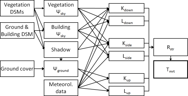
SOLWEIG is a model that simulates spatial variations of 3D radiation
fluxes and the Tmrt in complex urban settings. It is also able
to model spatial variations of shadow patterns. Tmrt is one of
the key meteorological variables governing human energy balance and the
thermal comfort of people. It is derived from summing all the radiative
(shortwave and longwave) fluxes (both direct and reflected) to which the
human body is exposed. In SOLWEIG, Tmrt is derived by modelling
shortwave and longwave radiation fluxes in six directions (upward,
downward and from the four cardinal points) and angular factors.
The model requires meteorological forcing data (global shortwave
radiation (Kdown), air temperature (Ta), relative humidity (RH)),
urban geometry (DSMs), and geographic information (latitude, longitude
and elevation). To determine Tmrt, continuous maps of sky view
factors are required. Both vegetation and ground cover information can
be added to increase the accuracy of the model output. Below,
a schematic flowchart of SOLWEIG in shown. The full
manual provides more
detail.
UMEP is a Python plugin used in conjunction with
QGIS. To install the software and the UMEP
plugin see the getting
started
section in the UMEP manual.
As UMEP is under constant development, some documentation may be missing
and/or there may be instability. Please report any issues or suggestions
to our repository.
The UMEP tutorial datasets can be downloaded from our here repository
here.
Download, extract and add the raster layers (DSM, CDSM, DEM and land
cover) from the input_dataset folder into a new QGIS session (see
below).
Create a new project
Examine the geodata by adding the layers (dsm_rotterdam,
cdsm_rotterdam, dem_rotterdam and lc_rotterdam) to your project (*Layer
> Add Layer > Add Raster Layer or drag and drop).
Coordinate system of the grids is Amersfoort / RD New (EPSG:28992). If you
look at the lower right hand side you can see the CRS used in the
current QGIS project.
Examine the different datasets before you move on.
To add a legend to the land cover raster you can load
landcoverstyle.qml found in the test dataset. Right click on the
land cover (Properties -> Style (lower left) -> Load Style).
Details of the model inputs and outputs are provided in the SOLWEIG
manual. As this tutorial is
concerned with a simple application only the most critical
parameters are used. Many other parameters can be modified to more
appropriate values, if applicable. The table below provides an overview
of the parameters that can be modified in the Simple application of
SOLWEIG.
Data use and type abbreviations:
R: required, O: Optional, N : not needed,
S: Spatial, M: Meteorological,
Influences solar related calculations. Set in the interface of the model.
Human exposure parameters
Absorption of radiation and posture
R
O
Set in the interface of the model.
Environmental parameters
e.g. albedos and emissivites of surrounding urban fabrics
R
O
Set in the interface of the model.
Meterological input data should be in UMEP format. You can use the
Meterological Preprocessor
to prepare your input data. It is also possible use the plugin for a single point in time.
Required meteorological data to calculate Tmrt are:
Air temperature (°C)
Relative humidity (%)
Incoming shortwave radiation (W m2)
The model performance will increase if diffuse and direct beam solar radiation is
available but the model can also calculate these variables.
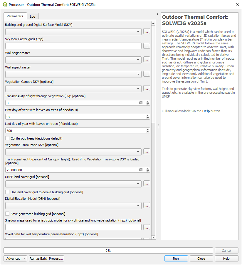
Open SOLWEIG in the Processing Toolbox from UMEP -> Processor -> Outdoor Thermal Comfort:
SOLWEIG v2025a.
You will make use of a test dataset from observations for Rotterdam, The Netherlands.
Dialog for the SOLWEIG model (click on figure for larger image)
To be able to run the model, some additional spatial datasets needs to
be created.
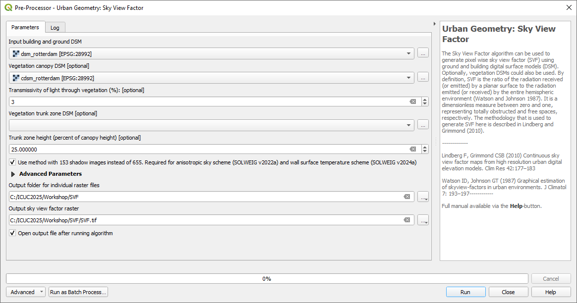
Close the SOLWEIG plugin and open UMEP from the processing toolbox then
Pre-Processor -> Urban geometry: Sky View Factor.
To run SOLWEIG various sky view factor (SVF) maps for both
vegetation and buildings must be created (see Lindberg and
Grimmond
(2011)
for details).
You can create all SVFs needed (vegetation and buildings) at the
same time. Use the settings as shown below. Use an appropriate
output folder for your computer.
When the calculation is done, a map will appear in the map canvas.
This is the ‘total’ SVF i.e., including both buildings and
vegetation. Examine the dataset.
Where are the highest and lowest values found?
If you look in your output folder you will find a zip-file containing all the
necessary SVF maps needed to run the SOLWEIG-model.
Another pre-processing plugin is needed to create the building wall
heights and aspect. Open UMEP from the processing toolbox again and then
Pre-Processor -> Urban geometry: Wall height and aspect and use the settings as shown below. QGIS scales loaded rasters by a cumulative count out approach
(98%). As the height and aspect layers are filled with zeros where no wall are present it might appear as if there is no walls identified. Rescale your
results to see the walls identified (Layer Properties > Symbology).
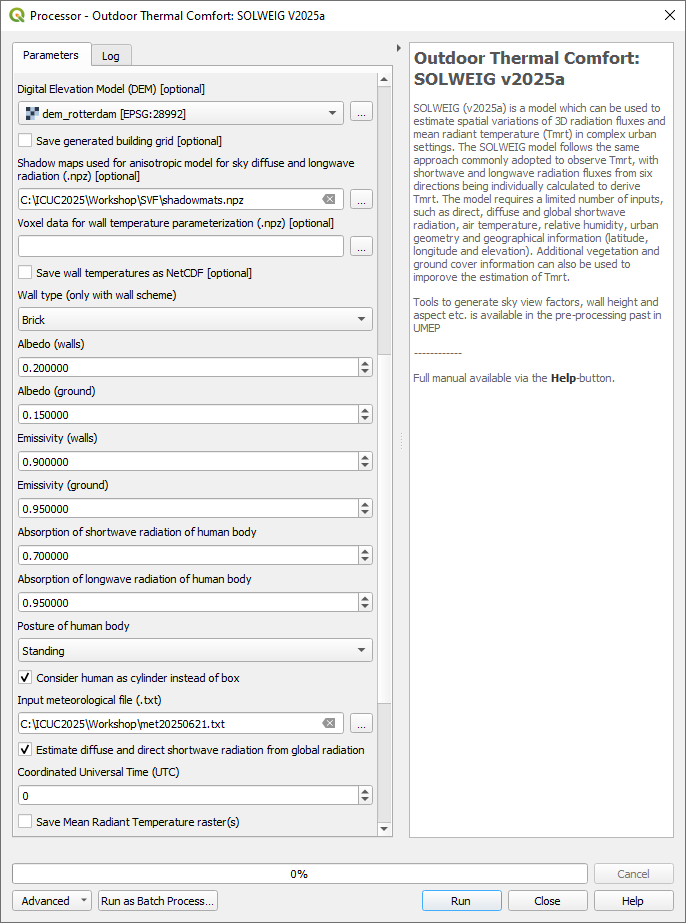
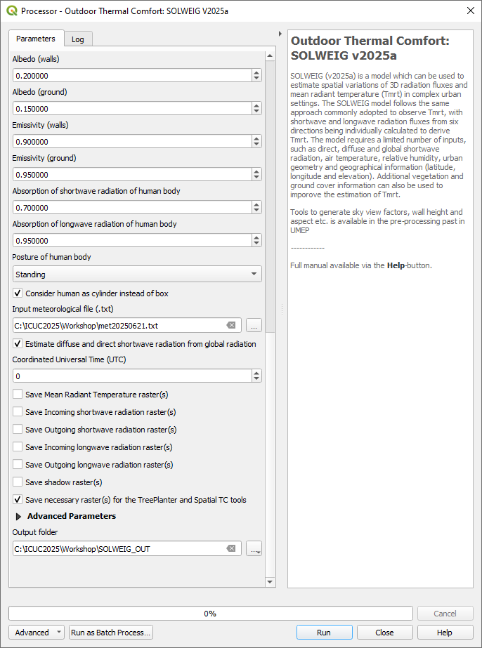
Re-open the SOLWEIG plugin and use the settings shown below.
You will use vegetation (cdsm_rotterdam.tif) and ground cover (lc_rotterdam.tif).
As no TDSM exists we estimate it by using 25% of the canopy height. Leave the tranmissivity as 3%.
You will use meteorological forcing data from KNMI (Royal Netherlands Meteorological Institute).
This data is in UTC 0. The solar radiation is global and therefore we have to tick “Estimate diffuse
and direct shortwave radiation from global radiation”. Remember to tick “Save necessary raster(s) for the TreePlanter and Spatial TC tools”.
Specify an output folder that you can easily find. Click Run.
The settings for your first SOLWEIG run (part 1) (click on figure for larger image).
The settings for your first SOLWEIG run (part 2) (click on figure for larger image).
The settings for your first SOLWEIG run (part 3) (click on figure for larger image).
Add the Tmrt_average.tif from your output folder and examine it (Average Tmrt (°C). What is the main
driver to the spatial variations in Tmrt?
Now add the Tmrt_2025_172_1200D.tif from the output folder. This file will be used later in the tutorial.
In this tutorial you will make use the model URock to estimate wind fields in an urban setting using a semi-empirical wind model based on Röckle (1990).
URock can be used to calculate the 3D wind field of an urban area using information about the wind (at least speed and direction at a given height) and geographical data describing the area of interest (building and vegetation footprint and height). Two main stages are used: wind field initialization and wind field balance. For a detailed description of the model see, Bernard et al. (2023).
The model requires meteorological forcing data (wind speed and direction) and geometry information for buildings and trees.
UMEP for Processing is a Python plugin used in conjunction with
QGIS. To install the software and the UMEP
plugin (if not already installed), see the getting started
section in the UMEP manual.
As UMEP for Processing is under constant development, some documentation may be missing
and/or there may be instability. Please report any issues or suggestions
to our repository.
We will use the DSM, CDSM and DEM that we used to force SOLWEIG. We, however, have to add another file; BuildingsRotterdam.gpkg that should also be in your input dataset.
To run URock, you need a building vector dataset including building height attributes and/or a vegetation vector layer including height and some additional optional info such as attenuation factor (see below). Here, you will make use of raster DSM, DEM and CDSM to generate information for URock.
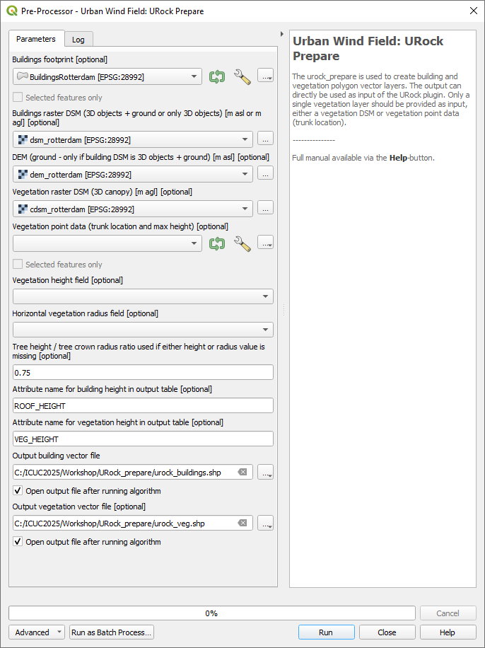
Open URock Prepare from the Pre-Processing section in UMEP for Processing found in the Processing Toolbox.
Use the settings shown below except for the output where you maybe need to specify a specific location on your computer where you have read and write access.
If you have a dataset with points including tree location and attributes with heights and/or ratio information, this can also be used to generate vegetation data. Now click Run and two new files that are ready to use in URock will be created. The current version of URock does not include ground topography (hopefully available in upcoming versions). The DEM is used to derive building heights comparing the DSM and the DEM.
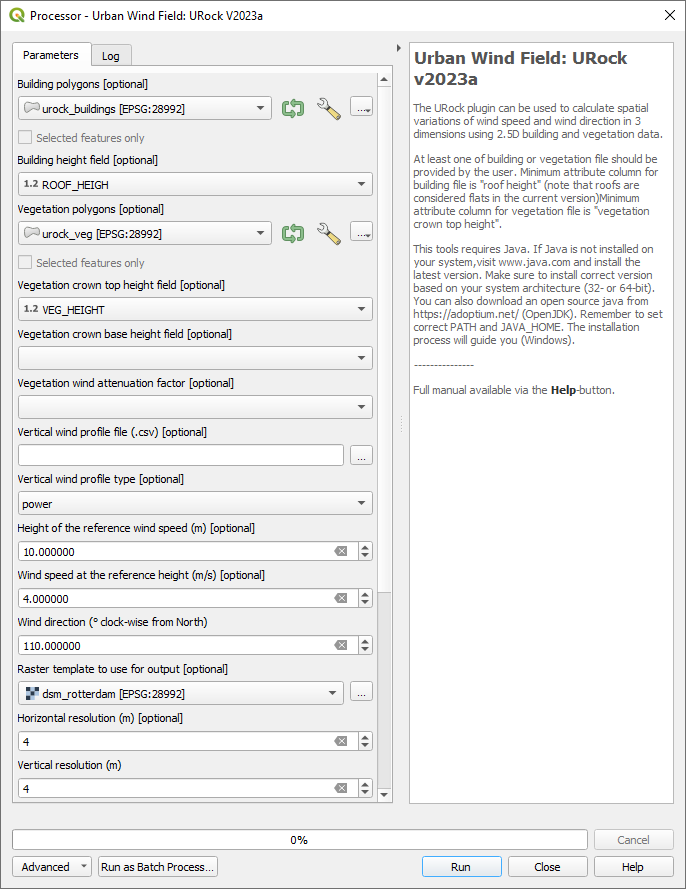
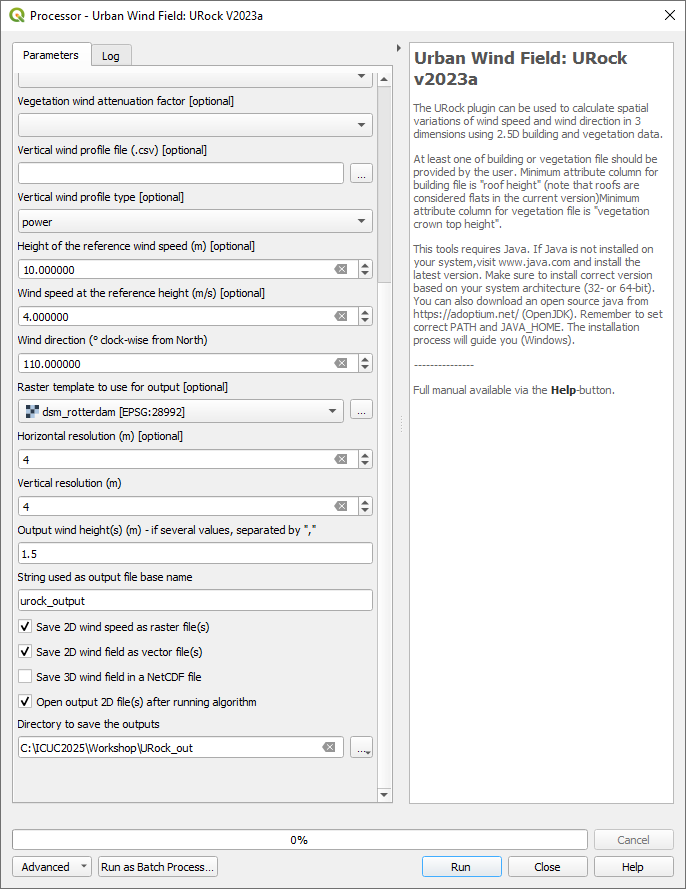
Open the URock interface (UMEP > Processing > Urban Wind Field: URock). Here you can make a lot of settings (divided into two figures).
We will use a wind speed of 4 m/s with a wind direction set to 110 degrees. To increase the speed of the calculations we will use 4 meter horizontal and vertical resolutions.
When all the settings are made, click Run.
The computation will take some time depending on your computer standard. During the computation, you can follow the steps in the log-window in the URock-interface. A large part of the computation time is related to creation of all the different zones around buildings and vegetation. If you want an even more detailed picture of the process, open the Python Console in QGIS. However, this will somehow slow down the computational process. When the computation is finished, the tool will load the raster windspeed and the vector points at 1.5 meter above ground level.
In this last step of the tutorial you will use the SpatialTC tool to produce maps of thermal comfort indices using outputs from the two previous steps (SOLWEIG and URock).
The two previous modeling steps provided us with Tmrt (SOLWEIG) and wind fields (URock). These outputs are combined in the SpatialTC-tool to generate raster maps on thermal indices such as PET, UTCI and COMFA.
Produce map of Universal Thermal Climate Index (UTCI) with SpatialTC
You need to specify two rasters: one of the mean radiant temperature that has been produced by SOLWEIG (Tmrt_2025_172_1200D.tif) and one with the pedestrian wind speed produced by URock (urock_outputWS.tif).
Load the Tmrt_2025_172_1200D.tif into your QGIS project if you have not done this already. This file can be found in your outout folder form the previous SOLWEG-run. Do not change the file name or its location as the info in the name will be used to identify the meteorological information that is needed to calcualte PET.
Last you need to select the thermal comfort index to map (UTCI for this tutorial). The Advanced parameters describing the person to consider for the comfort index (PET or COMFA) can also be defined but the default values are kept for this tutorial. Then click Run.